Pylon Benchmark
Motivation
The purpose of this benchmark is to show the influence of several types of stochastic loading on the stiffness and total strain energy, as well as to give some fundamental guidance on how to apply stochastic boundary conditions. To this end, we will be using and reusing an illustrative example that is easy to understand.
Key Takeaways
1. Deterministic performance
With equivalent model setups, a stochastically optimized part will have worse performance than a deterministic one in terms of stiffness and strain energy for the deterministic load case. This is simply a result of a fixed amount of mass available to the optimizer: the stochastic loading conditions ensure that material is distributed to make the part robust for many different loading conditions outside of the deterministic load case.
2. Non-deterministic performance
The stochastically optimized designs do have a significantly better stiffness performance for even small deviations from the deterministic load (see for example benchmark 3 : for any load that deviates more than three degrees from the nominal deterministic load, the stochastic shapes perform better than the deterministic one in terms of stiffness and strain energy).
3. Safety factor
We can mitigate the drop in deterministic stiffness by increasing the volume (and therefore mass) that the topology optimizer has available. This is not dissimilar to applying a safety factor (where it matters). See benchmark 2 for details.
4. Variation
Introducing too much stochastic variation (high standard deviations (normal distributions) or maximum angles (uniform distributions)) can have a detrimental effect on the stiffness without providing obvious benefits (note the 45-degree case in benchmark 1).
5. Load directions
The optimizer should apply material only where it is needed, which is why there are in principle two types of stochastic load scenarios: three-dimensional (where the direction of the load vector is free to vary in space) and two-dimensional (where the direction of the load vector varies on a defined plane). An appropriate selection of stochastic loading is a modelling choice like any other and needs to be carefully considered.
Summary of Benchmarks
We will present the following four benchmarks:
- Fixed volume target. Three-dimensional truncated normal distribution with varying standard deviation.
- Varying volume target. Three-dimensional truncated normal distribution with varying standard deviation.
- Fixed volume target. Two-dimensional uniform distribution with varying cut-off angles.
- Fixed volume target. Two-dimensional truncated normal distribution with varying standard deviation.
Design space and model setup
To highlight the stochastic aspect, the model presented here is quite simple. The design space is a cuboid with a zero displacement boundary condition on the bottom surface. It has a vertical load acting on the circular set on the top surface.
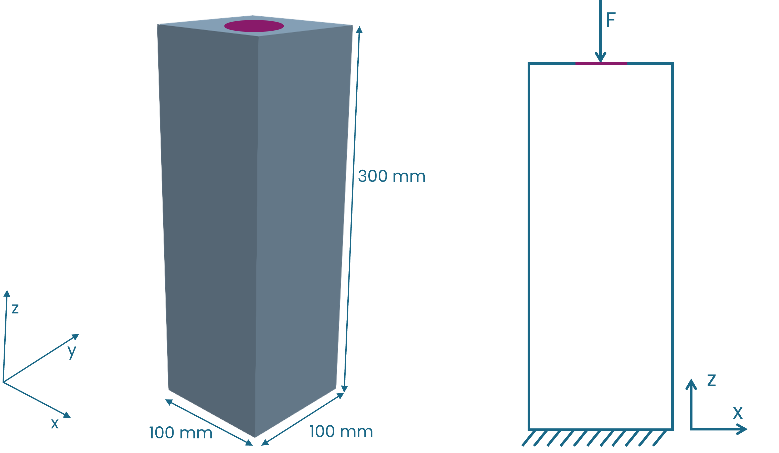
Fig. 1 Visualization of the design space (left) and the boundary conditions (right).
To make the stochastic benchmarks as comparable as possible, we chose a global model setup (as applicable to the individual benchmark. For example, the second benchmark does not have a fixed volume target).
Volume target: 10%
Mesh:
Initial mesh resolution: 20 (mesh size 8mm).
- Adaptive refinement strategy:
Maximum refinement levels: 3.
Maximum node increase: 10.
Anisotropic refinement (high quality surface pass).
- Boundary Conditions
Vertical load \(F = [0N, 0N, -100N]\) applied to the circular top surface.
Zero displacement applied at the bottom square surface.
- Stochastics:
three-dimensional distribution (
random_vector): resolution = 5 (21 points).two-dimensional distribution (truncated normal or uniform) (
random_disk): resolution = 21 (21 points).cut-off for the truncated normal distribution: max_angle = min_angle = \(90^\circ\).
stochastic loads have varying direction but constant magnitude.
Constraints: Keep Material thickness of 1 mm on the load surface.
Solver: max_iterations = 100.
Methodology
We performed each benchmark in two parts. First, we did several topology optimizations, applying a varying stochastic load. In a second step we then calculated stiffness and strain energy for each of the topology optimized shapes at certain deterministic loads, including the nominal load itself. Fig. 2 shows a schematic of the applied deterministic loads in relation to the nominal load.
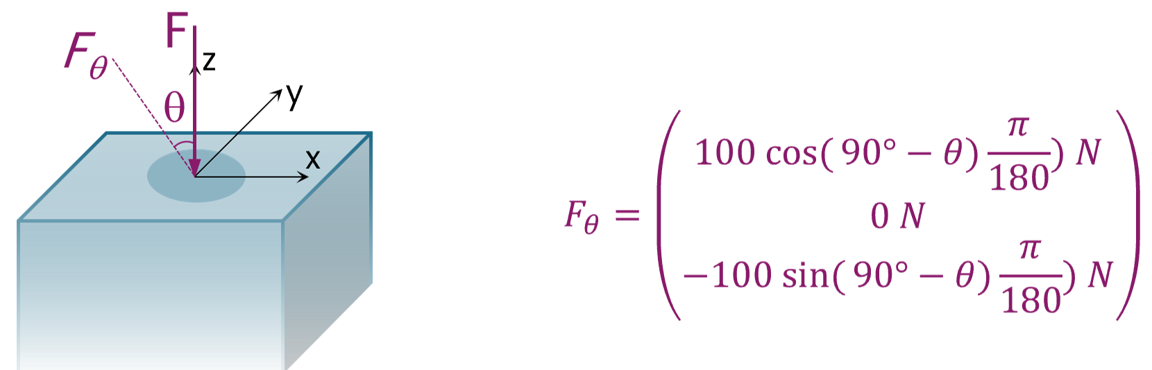
Fig. 2 Applied deterministic loads \(F_{\theta}\) with respect to nominal load \(F\).
Even though it is not technically correct, for the sake of brevity we will subsequently refer to the truncated normal distributions simply as normal distributions.
Benchmark 1: Three-dimensional distribution
For this benchmark, we performed the topology optimization with five different standard deviations \(\sigma\): \(1^\circ\), \(5^\circ\), \(10^\circ\), \(20^\circ\), and \(45^\circ\). The model setup is as described in the previous paragraph.
Summary and Conclusions
The deterministic design offers inferior performance with respect to stiffness for any non-deterministic load above 3 degrees compared to all other designs.
Large standard deviations (20 degrees and greater) in the topology optimization have a particularly detrimental effect on the stiffness for loads at smaller angles (up to 10 degrees), which is not balanced out by better performance for larger angles.
Results
Fig. 3 shows the resulting shapes. In this range of standard deviations there are three distinct shapes: for the deterministic case and a small standard deviation of \(1^\circ\), the shape has the form of a pillar since the acting force is mainly vertical. With increasing standard deviation and therefore increasing loads acting at an angle, the shape develops four legs ( \(\sigma\) = \(5^\circ\) and \(\sigma\) = \(10^\circ\)). As \(\sigma\) increases, additional reinforcements develop between these legs (\(\sigma\) = \(20^\circ\) and \(\sigma\) = \(45^\circ\)). The bifurcations or ‘jumps’ of the shape types thus occur between 1 and 5 degrees and then again between 10 and 20 degrees.
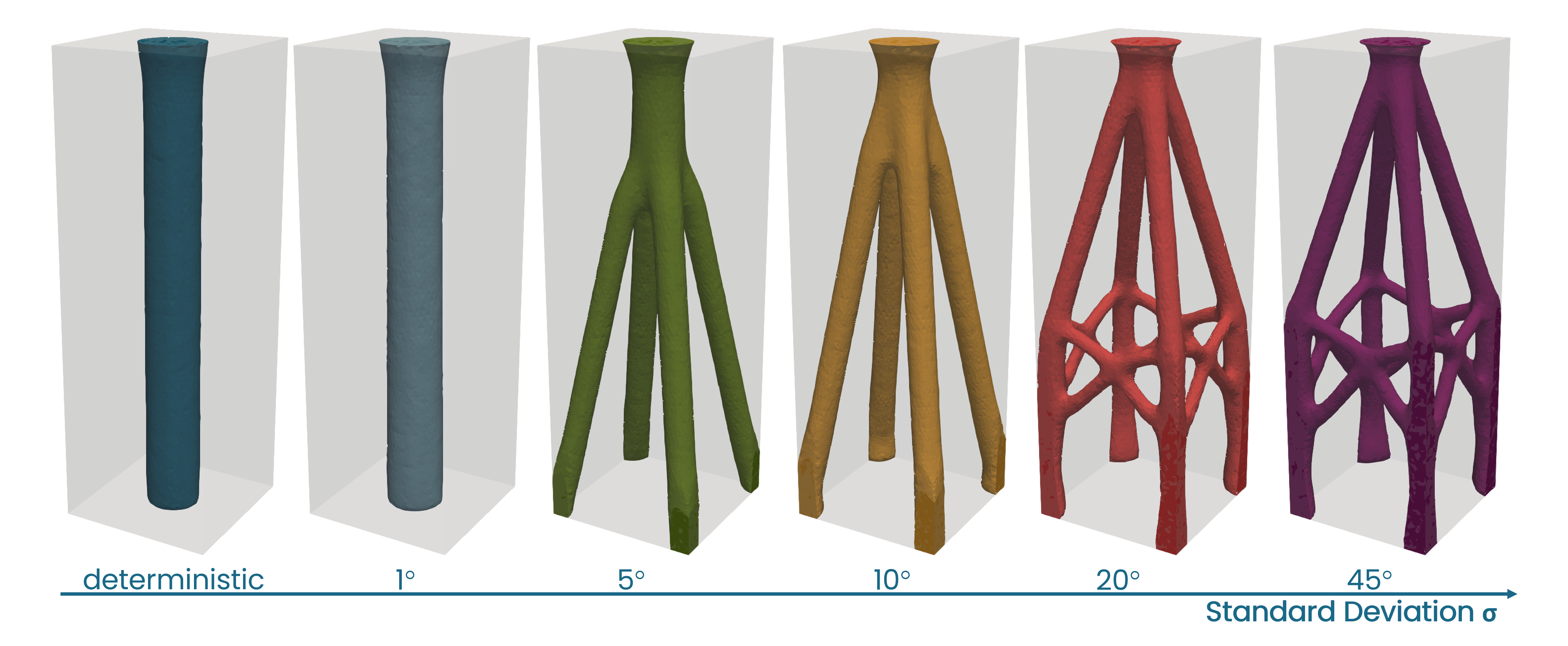
Fig. 3 Optimized shapes for different standard deviations \(\sigma\) , three-dimensional distribution.
Fig. 4 and Fig. 5 show the stiffness and total strain energy respectively for a spectrum of deterministic loads, characterized by the angle theta as shown in Fig. 2. For all designs, the stiffness decreases monotonically as the load \(F_{\theta}\) deviates from the nominal \(F\).
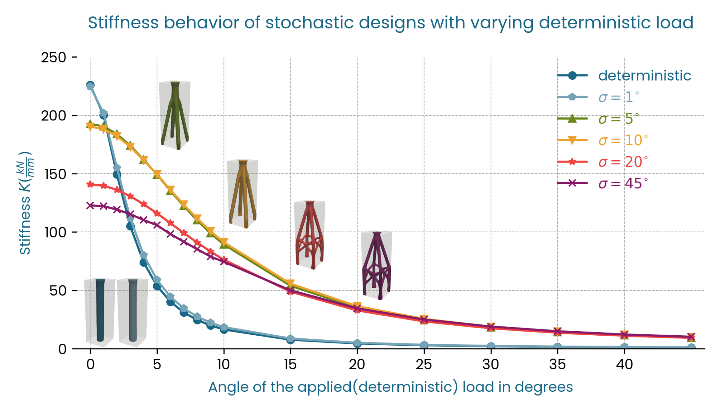
Fig. 4 Stiffness \(K\) vs \(F_{\theta}\), three-dimensional distribution, resolution 5.
We observe the same robustness trend when considering the strain energy as seen in Fig. 5.
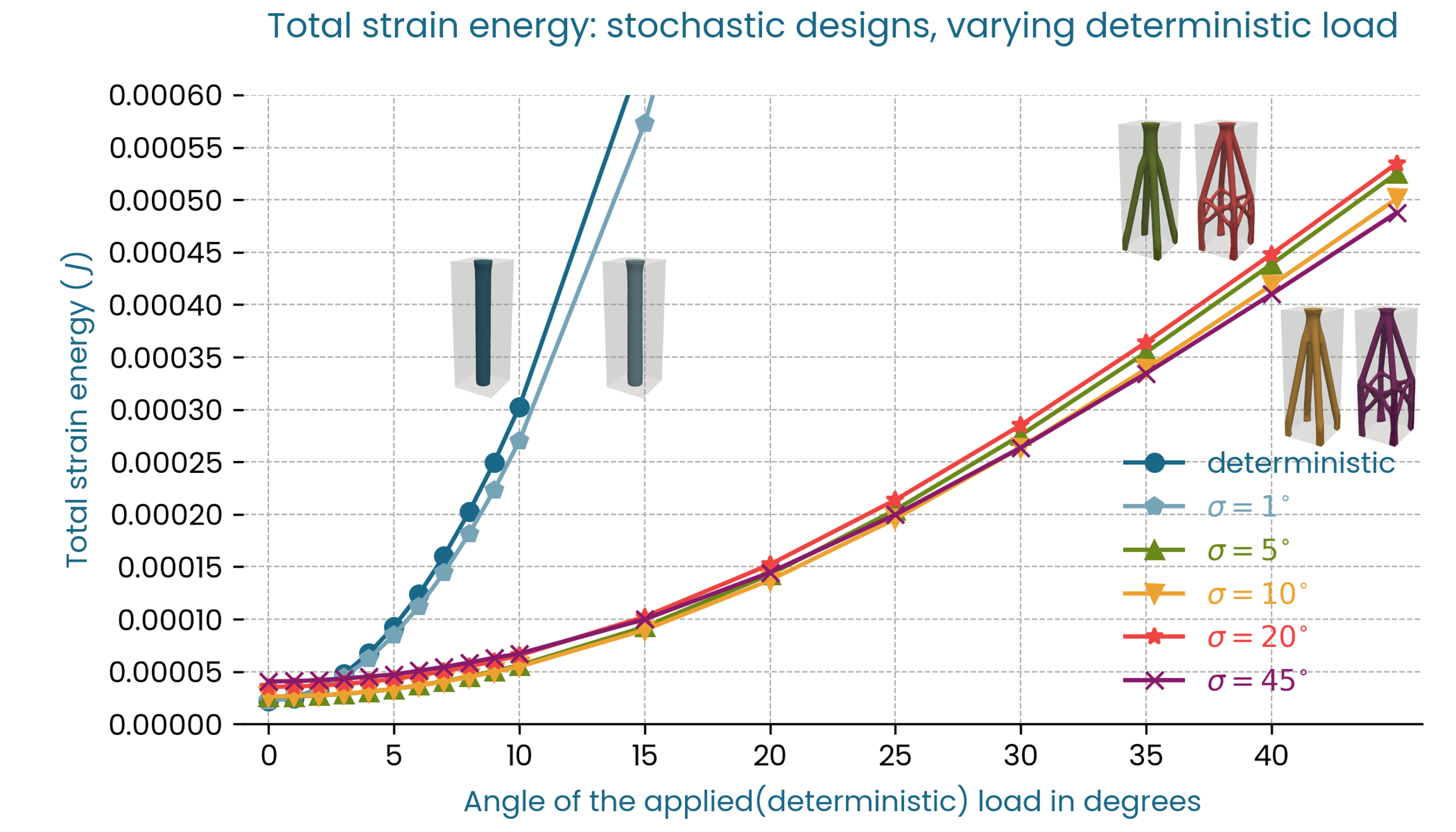
Fig. 5 Strain Energy \(U\) vs \(F_{\theta}\), three-dimensional distribution, resolution 5.
The deterministic and low standard deviation designs offer worse performance for \(\theta > 3^\circ\) than the stochastic designs with higher standard deviations both in terms of stiffness, and total strain energy. In this case, in terms of stiffness the optimal standard deviations to achieve a robust design that performs well on the full range of loads are in the middle range: \(\sigma\) = \(5^\circ\) and \(\sigma\) = \(10^\circ\), since these designs have a less pronounced stiffness drop compared to the designs with higher standard deviations, with similar performance for the tail loads.
It is clear from this benchmark that with a constant volume and hence weight target, the stiffness of the stochastic designs decreases for the deterministic loadcase, and that there is a higher drop in initial stiffness for designs with higher standard deviations. This makes sense, since a greater standard deviation means a greater spread in loading conditions that the design is subjected to during the optimization. The available material must be distributed by the solver in a way that accounts for a more diverse load envelope.
Benchmark 2: Varying volume target with a three-dimensional distribution
The purpose of this benchmark is to demonstrate how it is possible to meet a deterministic stiffness target by increasing the volume target in a stochastic setting and to quantify this increase for the pylon example. Another way of thinking about this is that increasing the weight target is not dissimilar to applying a safety factor. The optimizer can distribute this additional weight in a coordinated way. As in the previous benchmark we performed the topology optimization with the three-dimensional stochastic load, but only four different standard deviations \(5^\circ\), \(10^\circ\), \(20^\circ\), and \(45^\circ\). The model setup is nearly identical to the previous benchmark, but in addition to varying the standard deviation we also varied the volume target. As well as the original 10%, we conducted optimizations for 12%, 15% and 20%. We then calculated the stiffness and strain energy for each of these designs at the deterministic nominal load \(F\).
Summary and Conclusions
Adding mass can change the quality of a shape (demonstrated by the shapes for 20 degrees standard deviation)
Changing the volume target is not dissimilar to applying a safety factor to the design in a (hopefully more intelligent) way
Both stiffness and strain energy improve monotonically with increasing weight.
Results
Fig. 6 shows the optimized shapes. Interestingly, for a standard deviation of \(20^\circ\) the type of the shape changes as the volume target increases from 12% to 15% and it jumps from having additional reinforcements between the legs to no reinforcements.
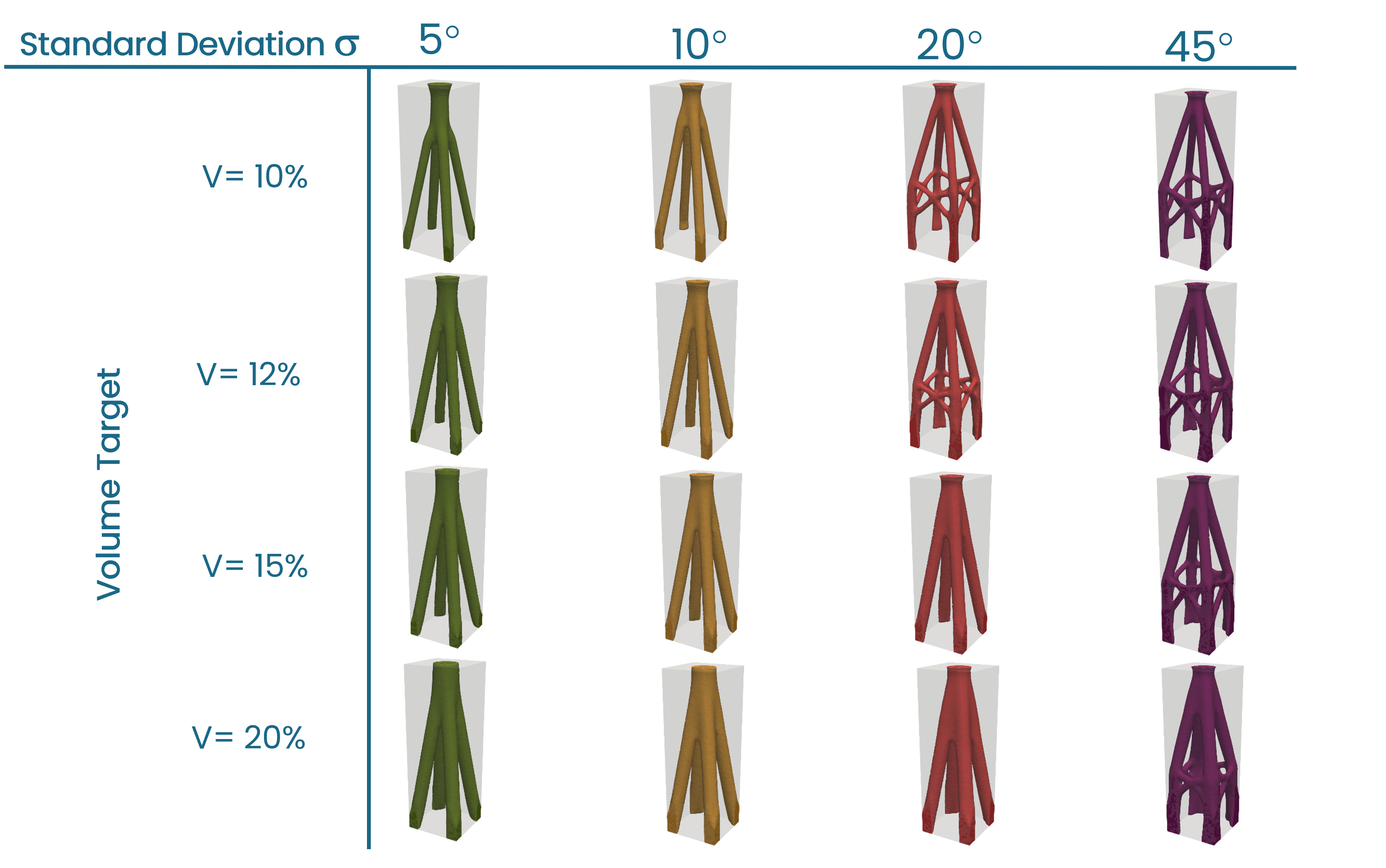
Fig. 6 Optimized shapes for different standard deviations \(\sigma\) , three-dimensional distribution.
First, the stiffness plot in Fig. 7 shows that, as expected, the stiffness at the nominal load increases with increasing volume target, so by making the shape heavier the original deterministic stiffness can be reached or exceeded. In this example an increase of around 20% would be sufficient for the smaller standard deviations of 5 and 10 degrees, while the weight has to increase by 50% to meet the original stiffness when the standard deviation is 45 degrees. In this case, the relationship between volume and stiffness is nearly linear apart from the case where the type of the shape changes (\(\sigma\) = \(20^\circ\)).
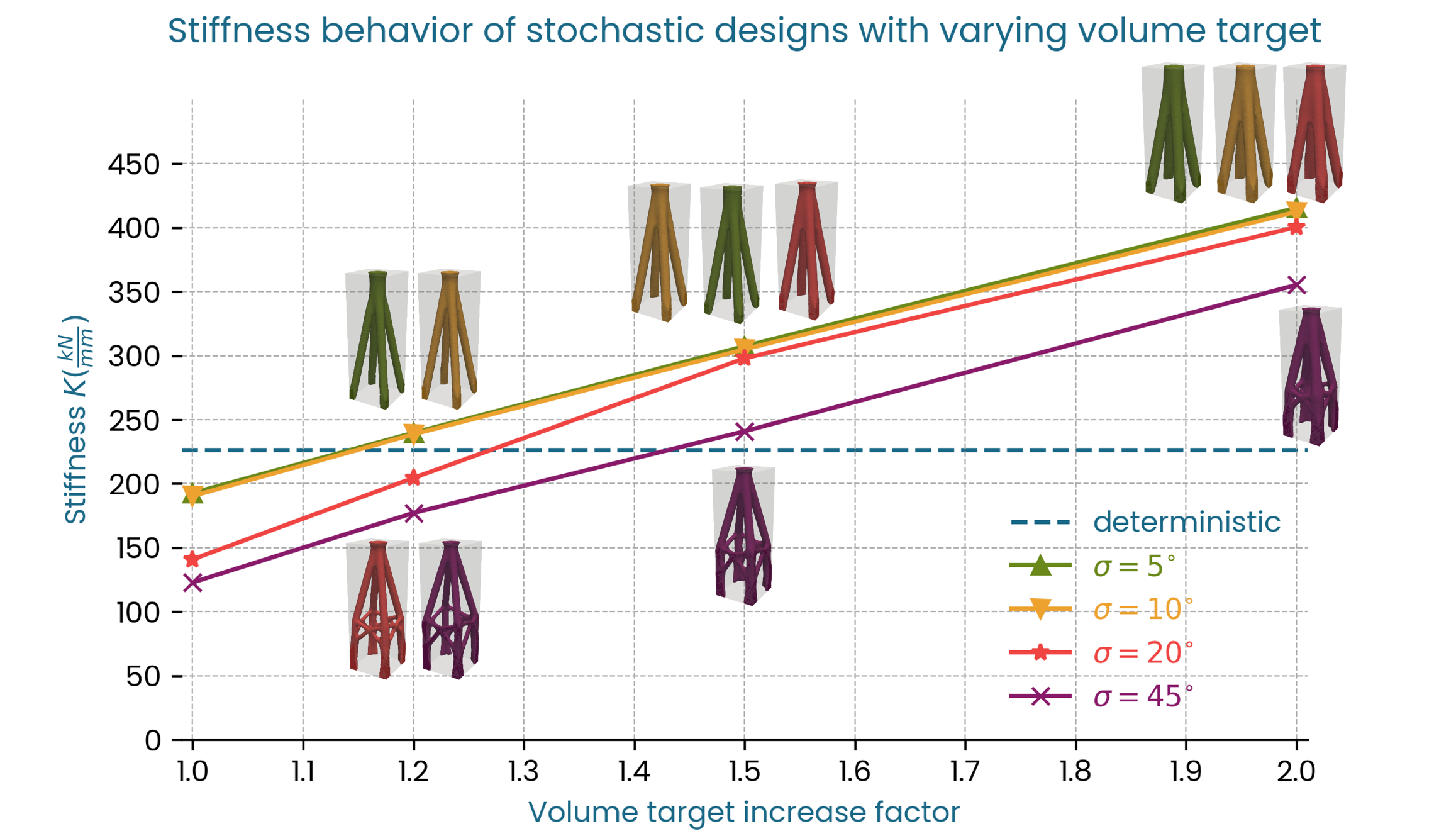
Fig. 7 Stiffness \(K\) vs Volume target, three-dimensional distribution.
We observe a similar trend for the total strain energy: at 20% volume increase the strain energy is below the deterministic case for standard deviations of 5, and 10 degrees, while the volume has to increase by close to 50% for the strain energy of the 45-degree shape to be below the strain energy of the deterministic case.
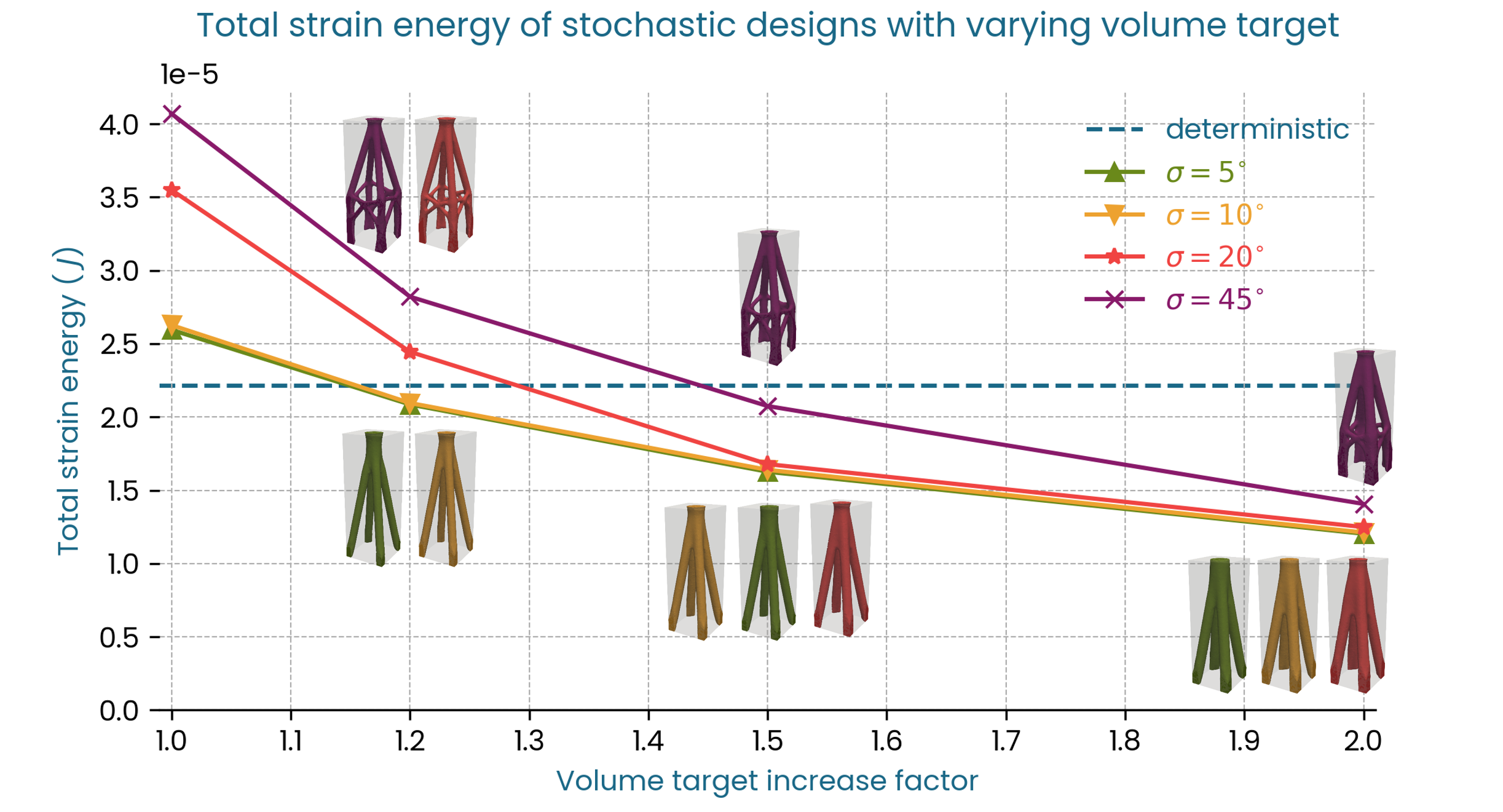
Fig. 8 Strain Energy \(U\) vs Volume target, three-dimensional distribution.
Benchmark 3: Uniform two-dimensional distribution
For many engineering problems load transfer is limited to specific directions. For such a problem, the previous three-dimensional load variation would be a bad modelling assumption, since the topology optimizer will distribute material where it is not required, because the loads that the optimized part was designed for do not actually occur in service.
In this benchmark, we limit the stochastic load distribution to the xz-plane (y=0). Except for the stochastic loading, the modelling setup is very similar to the first benchmark. For the stochastic loading, we assume a uniform distribution, which means that within a range of angles [\(\theta_{min}\), \(\theta_{max}\)] each load is equally likely to occur. We also chose the distribution to be symmetric about the central load, which means that max_angle and min_angle are related: \(\theta_{min} = -\theta_{max}\). Finally, since the previous benchmarks showed no clear benefit of employing large standard deviations \(\theta_{max} \in \{1^\circ, 5^\circ, 10^\circ, 15^\circ, 20^\circ\}\). It is important to be aware, that for the uniform distribution \(\theta_{max}\) is the cut-off angle so it corresponds to the most extreme load considered, while for the normal distribution from previous benchmarks, the standard deviation marks the interval of only about two thirds of all loads considered.
Summary and Conclusions
Two-dimensional distributions for same resolution are much cheaper computationally, for the same resolution (res 21 for a three-dimensional distribution would correspond to 421 samples).
The designs with the two-dimensional uniform distribution have a higher initial stiffness and a smaller drop in stiffness for increasing load angles.
Results
Fig. 9 shows the resulting shapes. It is quite clear from this figure that, as expected, the optimizer distributes the available material in the loading plane.
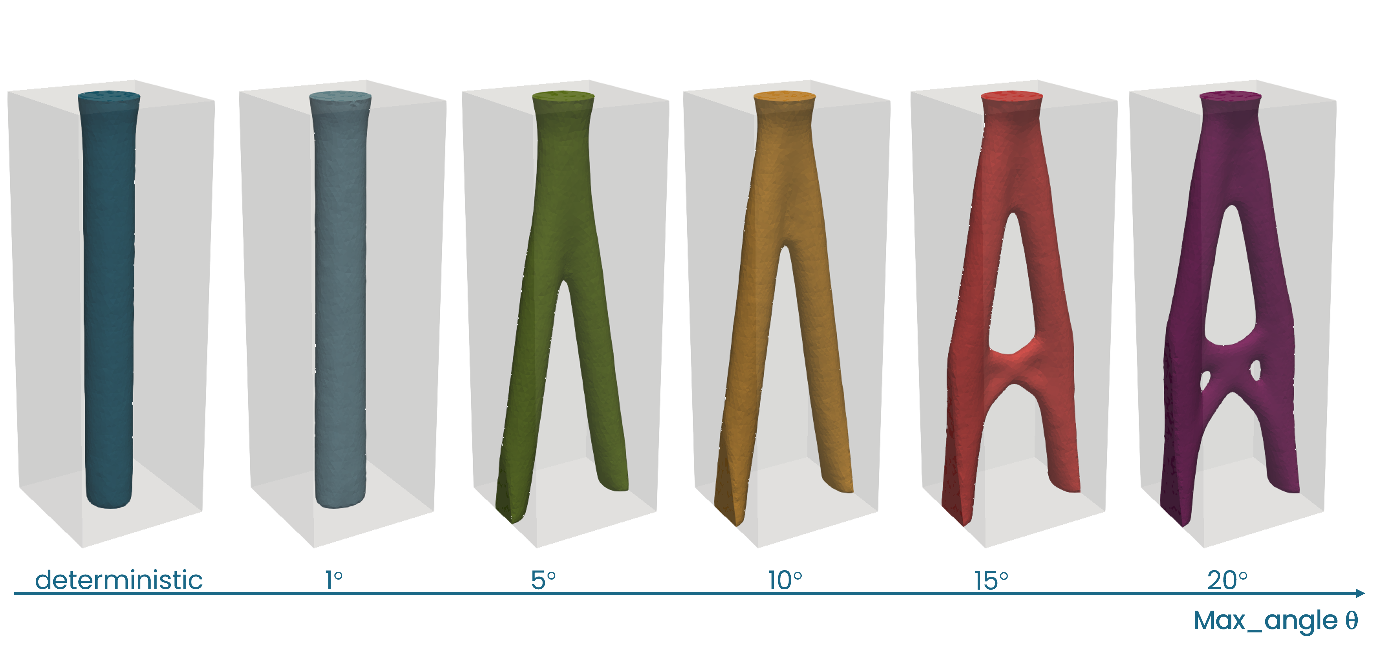
Fig. 9 Optimized shapes for different max_angle \(\theta_{max}\) , two-dimensional distribution.
Fig. 10 shows the stiffness behavior, where \(F_{\theta}\) acts in the xz-plane and is defined as before (Fig. 2). The stiffness shows a similar global trend to benchmark 1. However, when directly compared to the three-dimensional case, the drop in stiffness of the stochastic designs for the deterministic load (\(\theta = 0^\circ\)) is significantly lower. Also, for load angles greater than 5 degrees, the design with the highest cutoff-angle (\(\theta_{max} = 20^\circ\)) outperforms all other designs in terms of stiffness.
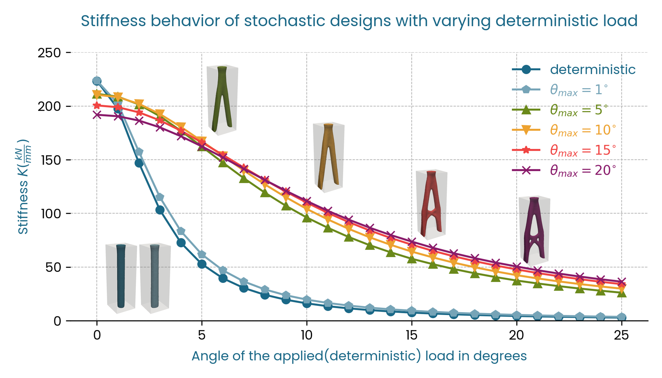
Fig. 10 Stiffness \(K\) vs \(F_{\theta}\), two-dimensional distribution.
Fig. 11 shows a similar trend for the total strain energy.
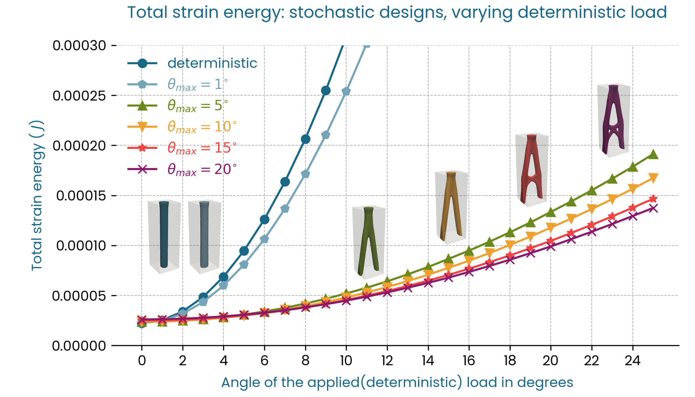
Fig. 11 Strain Energy \(U\) vs \(F_{\theta}\), two-dimensional distribution.
Benchmark 4: Normal two-dimensional distribution
As in the previous benchmark we performed the topology optimization with the two-dimensional stochastic load, but with a normal distribution rather than a uniform distribution and five standard deviations \(1^\circ\) \(5^\circ\), \(10^\circ\), \(15^\circ\), and \(20^\circ\). The model setup is otherwise identical to the previous benchmark. For the normal distribution, the loads are weighted. More extreme loads are assigned a lower weighting. Compared to the uniform distribution of benchmark 3 these settings correspond to a significantly higher spread in load cases. For example, the highest standard deviation \(\sigma = 20^\circ\) means that the actual cut-off angle for the load interval is around 40 degrees.
Summary and Conclusions
The designs with the two-dimensional normal distributions also have a higher initial stiffness and smaller drop for increasing load angles.
- Initial stiffness drops compared to the deterministic design for standard deviations 5, 10 and 20 degrees:
three-dimensional: -15%, -16%, -38%.
two-dimensional: -7%, -15%, -23%.
Results
The greater load variation explains the difference between the shapes for the normal distribution, shown in Fig. 12, and the uniform distribution in Fig. 9. Interestingly, for a standard deviation as low as 1 degree, the resulting shape already deviates from the deterministic pillar form, and as the standard deviation increases the cross-bar reinforcements disappear in favor of a closed surface.
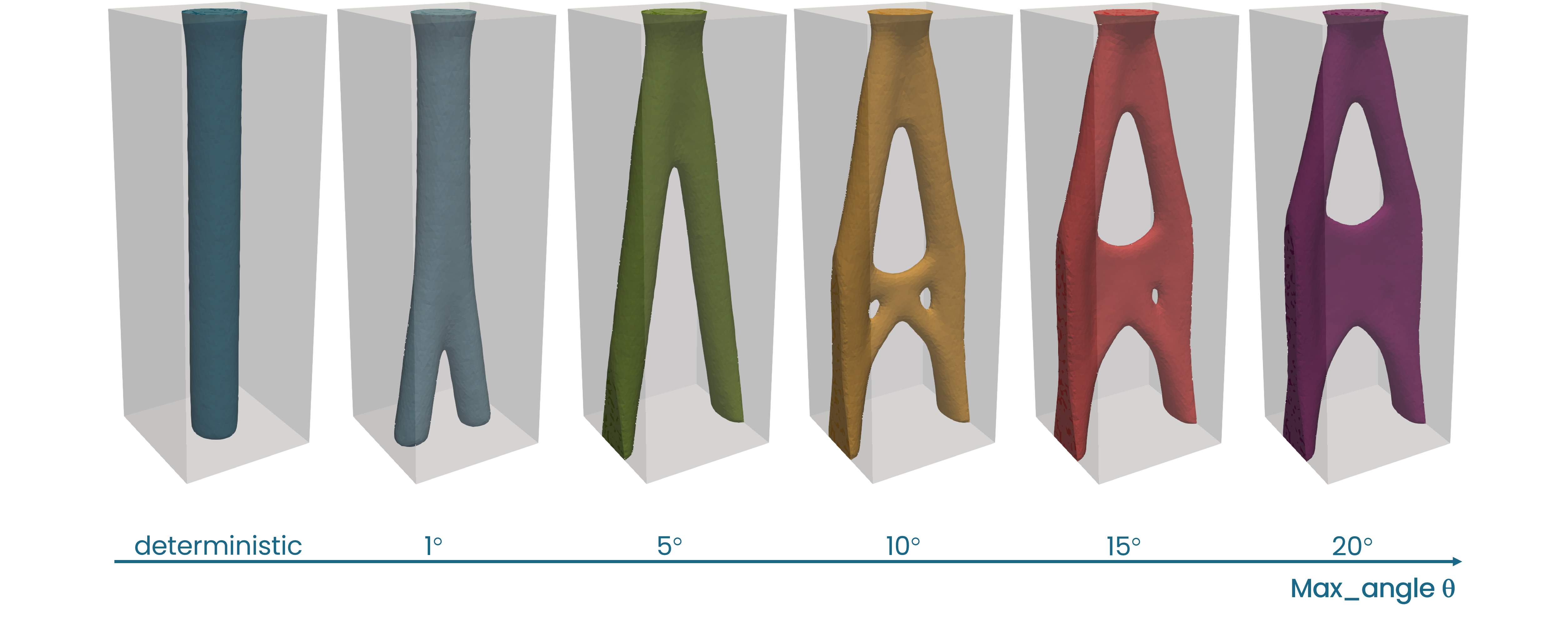
Fig. 12 Optimized shapes for different standard deviations \(\sigma\) , two-dimensional distribution.
In terms of stiffness (Fig. 13) and strain energy (Fig. 14) the optimized shapes follow a similar pattern to the previous benchmark, with the exception of \(\sigma = 1^\circ\) which is a hybrid in terms of shape and also exhibits an intermediate stiffness and strain energy behavior.
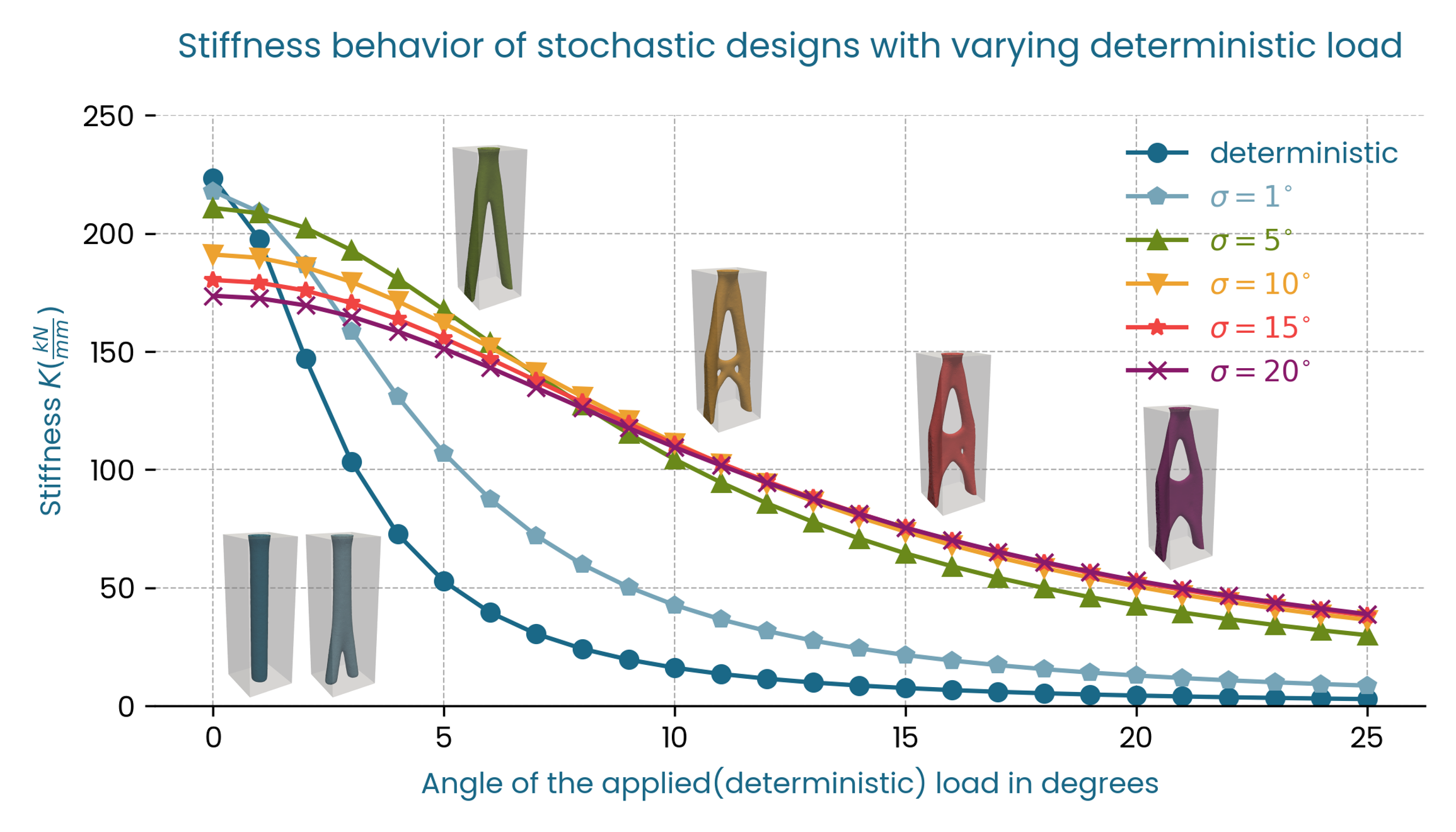
Fig. 13 Stiffness \(K\) vs \(F_{\theta}\), two-dimensional distribution.
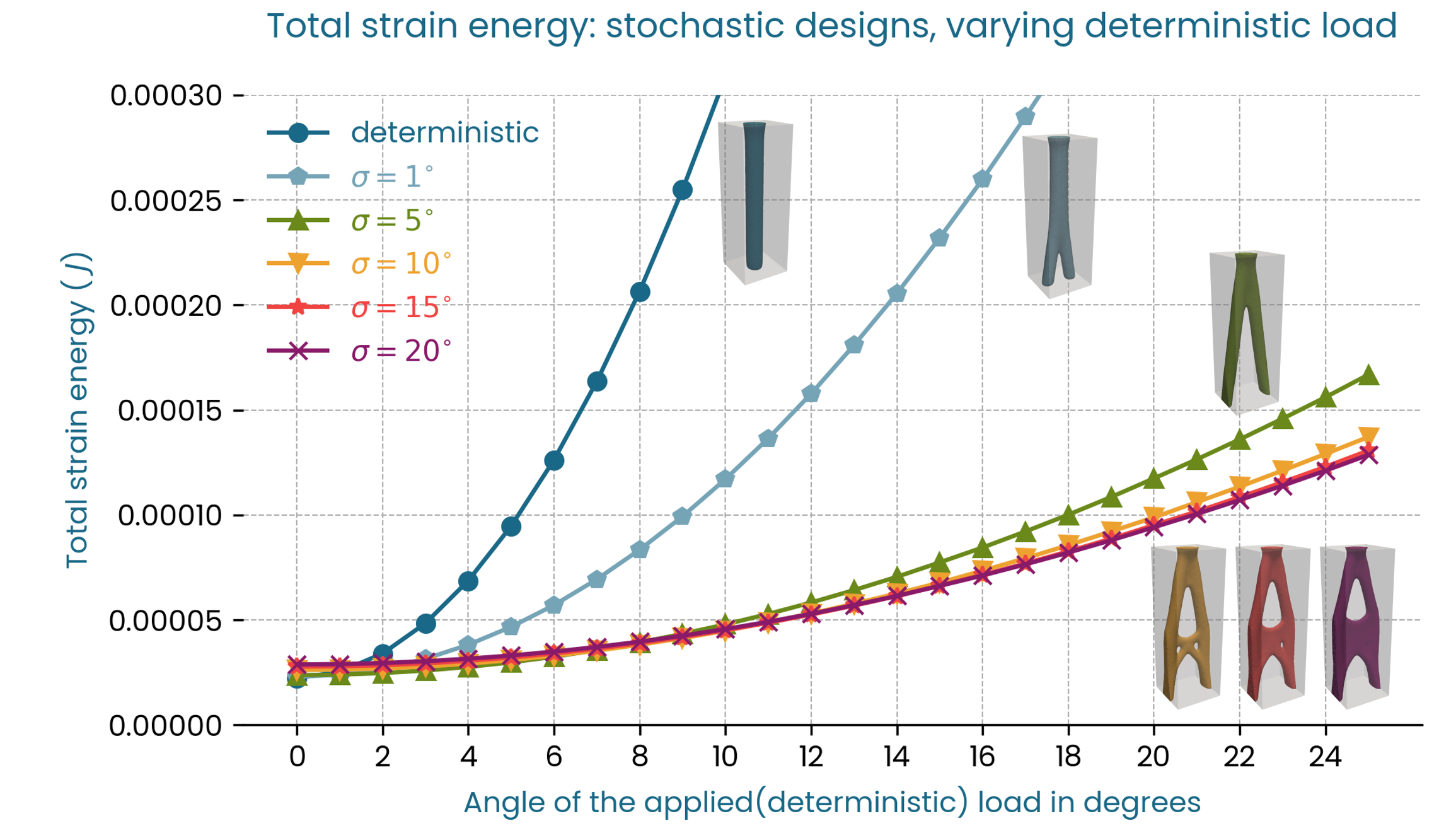
Fig. 14 Strain Energy \(U\) vs \(F_{\theta}\), two-dimensional distribution.