9. Connections
Connector elements allow for a more correct representation of loads, constraints, and connections between parts of an assembly.
There are three main types of connections: rigid and soft couplings, and springs. These connect different types of targets, as summarized in table Couplings and springs.
Couplings |
Springs |
|---|---|
|

|
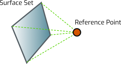
Couplings are defined between surface sets and reference points |
Springs are defined between two distinct reference points |
The Connections tree lists existing connections, together with the controls to create, edit, clone, or delete any of these entities.
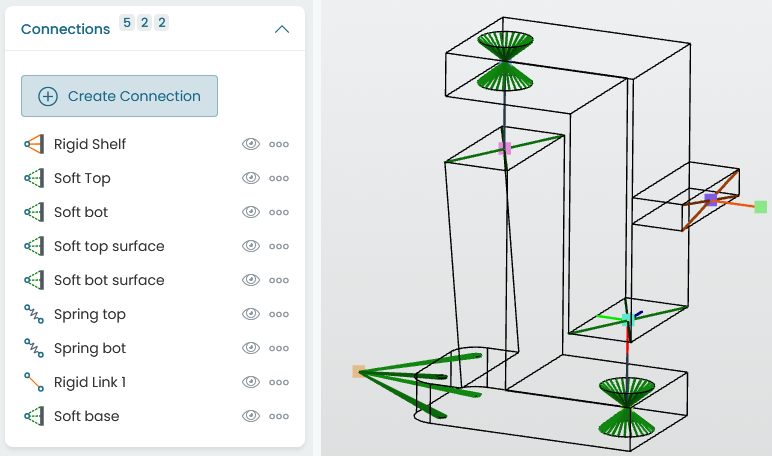
Fig. 9.1 Connections tree
Note
Connections (couplings and springs) are key to arrive to a realistic structural FEA representation of reality. They allow for much improved local constraints via couplings. Furthermore, the use of pairs of couplings connected via a zero length spring offers a general approach to model complex fasteners or bearings.
Therefore, it is recommended to spend time planning an FEA setup in terms of these elements in an assembly sense. This approach will allow the topology optimized results to be close to the physical structural application.
9.1. Couplings
Couplings create constraints between surface sets and reference points.
For all coupling types, Coupling properties include its name, control or reference point, and surface sets.
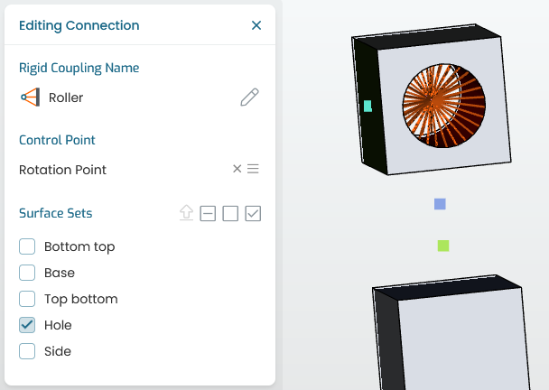
Fig. 9.2 Coupling properties
It is very important to understand the differences between rigid and soft couplings, in order to select the appropriate type to represent reality as close as possible.
Note
Rigid Coupling is equivalent to RBE2 in Nastran, or kinematic coupling in Abaqus.
Soft Coupling is equivalent to RBE3 in Nastran, or distributing coupling in Abaqus.
9.1.1. Rigid couplings
Rigid couplings are also known as kinematic couplings, or RBE2.
In this type of coupling, the reference point dictates the motion of all constrained surfaces. If creates an infinite stiffness between the nodes, not allowing relative motion between them. As a result, this local area is usually over-constrained and cannot be used for localized stress prediction.
These are often used for noise, vibration, and harshness (NVH) models, and areas where stresses are not of interest local to the attachment / coupling area.
9.1.2. Soft couplings
Soft couplings are also known as distributed couplings, or RBE3.
The reference point motion is dictated by the average of the nodes in the coupled surfaces. These couplings do not change the local or global stiffness. Local bending of the node-set is allowed, and therefore stress distributions will be more realistic in most cases.
These are mainly used for smooth application of loadings and constraints.
9.1.3. Rigid vs soft couplings
Fig. 9.3 presents a simple example comprising a simple geometry with two holes; the topology is optimized to minimize compliance. Each hole is connected to a reference point located at its center using rigid or soft couplings. The top reference point is then fixed, and the bottom is loaded vertically. No additional shape constrains are applied.
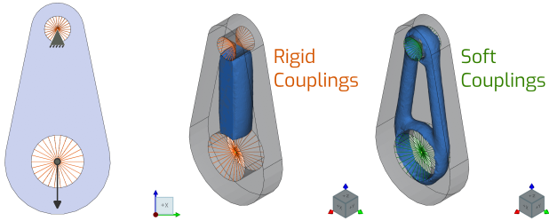
Fig. 9.3 Topology optimization problem considering rigid and soft couplings, and resulting optimized shapes.
The resulting optimized shapes clearly indicate the difference between the two types of couplings:
The rigid coupling is infinitely stiff, and therefore the two holes are connected with a single member;
The soft coupling models a softer distribution of the constraint and load. The shape is therefore more detailed around these holes.
Soft couplings are therefore the recommended method for topology optimization. The rigid type will likely over-constrain the set-up, and its use is discouraged within Möbius.
9.2. Springs
Springs are also known as linear elastic connectors, joints, or CBUSH elements.
These connect two reference points, each with 6 degrees of freedom (DOF), and are defined by 6 linear stiffness components — defined in global coordinates or a local coordinate system — applied to the relative displacement between the two points.
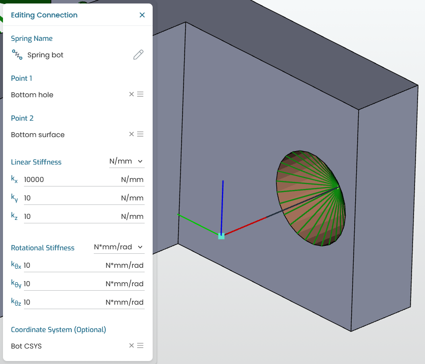
Fig. 9.4 Spring properties
If no coordinate system is specified, the orientation defined by the global coordinate system is used.
Typical applications of springs use either zero or high stiffness values per DOF to form joints: pinned, slider, tied, cylindrical, etc. For rigid-like, high-stiffness connections, linear stiffness values of \(1{\times}10^{6}\;\text{N/mm}\) and rotational stiffness values of \(1{\times}10^{8}\;\text{N}\,\text{mm}/\text{rad}\) are typical for most linear mechanical assemblies.
Furthermore, these elements can represent joints to parts or sub-assemblies not included in the model. These are replaced by springs between the model and a fully constrained node (reference point), with an appropriate stiffness. These are commonly referred to as spring-to-ground.
Tip
It is recommended for CAE teams to name reference points, couplings and springs with sensible names common to similar applications, or their function in the model. This should help to speed up workflows when it comes to adding loads, constraints and couplings.
Furthermore, the FEA (pre & validation) analysis in Möbius generates a text results file (CSV), which makes use of reference point names to report stiffness, displacement and reactions if a load (force or moment) or a constraint is applied to them.