13. Optimization Setup

13.1. Objective

The Objective panel allows defining a volume target for a maximize stiffness optimization. This can be done either as a percentage of the total design space volume(s) or by inputting the volume target with the correct units.

Furthermore, for multi-volume assemblies, this panel allows selecting the parts of the model to be optimized (design space volumes), given that they are represented by different volumes. By default, the solver will assume that all unselected volumes are non-design space, and form part of the assembly with their stiffness contribution, and any loads and / or constraints applied to them.

Fig. 13.1 shows a single volume model example.

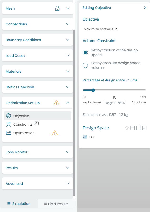
Fig. 13.1 Optimization objective

Hint

At the time of writing, the only optimization type available is maximize stiffness. Rafinex is currently preparing the release of a minimize mass (stress based) optimization.

13.2. Constraints

This panel allows applying optimization constraints, which are different from the model restraints covered under the Boundary Conditions section.

13.2.1. Symmetry

There are several symmetry options available in Möbius: plane, cyclic and point symmetry. In an assembly, it is possible to assign a different plane / axis symmetry constraint per volume.

Furthermore, plane symmetry constraints can be combined to form complex multi-axis conditions.

Fig. 13.2 shows an example for a single volume model.

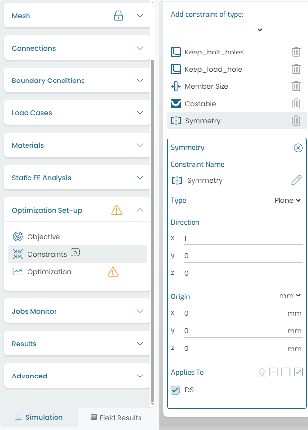
Fig. 13.2 Symmetry constraint

Note

If an existing symmetry type is not available in the User Interface, it can be applied via the Model Editor panel. Please contact Rafinex (support@rafinex.com) for further details.

13.2.2. Casting

In an assembly, it is possible to assign different axis casting constraints per volume. Casting draft angle is also supported by Möbius.

Fig. 13.3 shows an example for a single volume model.

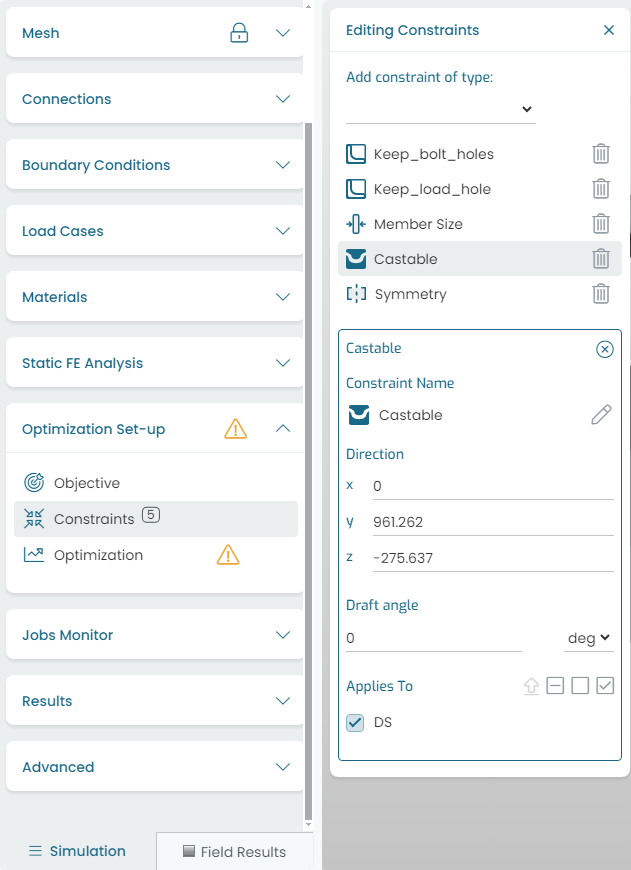
Fig. 13.3 Casting constraint

Fig. 13.4 shows an example of an assembly combining symmetry and casting constraints on a per-volume basis.

Fig. 13.4 Symmetry and casting constraints

13.2.3. Member Size

The Maximum Member Size constraint is supported in Möbius.

It is emphasized that this constraint is implemented in an automated manner (input mesh independent) in the solver. The direct benefit of this unique feature is that users do not need to input a fine mesh resolution, and / or perform trial and error runs with different mesh resolutions.

The solver will take care of the volume target value in combination with the maximum member size value set by the user, and through its adaptive remeshing technique, arrive to a sensible shape with the required final mesh resolution.

Fig. 13.5 shows an example for this constraint entry.

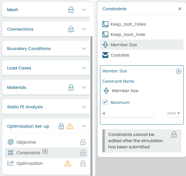
Fig. 13.5 Member size constraint

Warning

The member size constraint should be applied with care. If the model is of large dimensions, and the maximum member size value is small, the solver may generate very large meshes for the resolution to be adequate to the user’s input.

In these cases, default RAM limitations may apply; please contact Rafinex (support@rafinex.com) to increase cloud computing power for your account if required.

13.2.4. Keep Material Thickness

This constraint is applied on surface sets. It will apply a material thickness value, forming a volume of material treated as non-design space from the start of the optimization analysis.

This feature removes the need to split CAD models into several bodies when features like bolt bosses, walls or relatively small features need to be kept from the start of the optimization analysis.

Fig. 13.6 shows an example for this constraint entry.

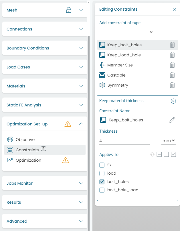
Fig. 13.6 Keep thickness constraint

13.2.5. Overhang

Möbius supports avoiding overhangs in the optimized shape. This type of constraint is of special importance for additive manufacturing methods, where it is often technologically impossible to layer the material beyond a certain slope limit without creating additional supports.

The Overhang constraint is defined by its Angle, the deposition (print) direction, a selection of Base Sets, and a selection of volumes where it will be applied.

Fig. 13.7 shows an example for this constraint entry.

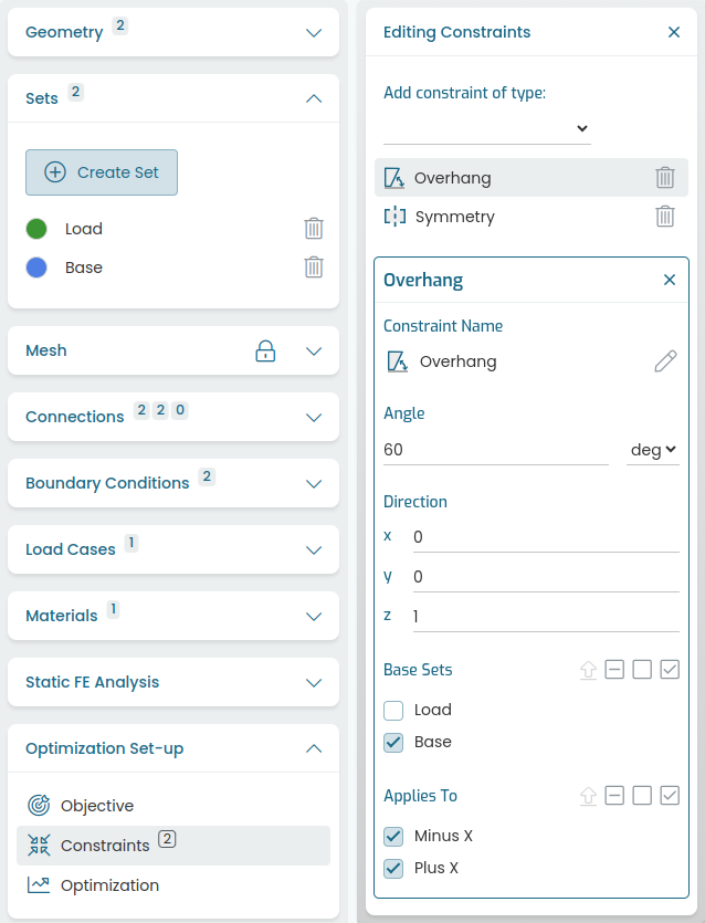
Fig. 13.7 Overhang constraint

Warning

Depending on the application, it might be necessary to include non-design space volumes to ensure correct overhangs detection in any design space volumes that may not be connected to the base.

Any overhangs in non-design space volumes will be left untouched, as no material can be removed from there.

13.2.5.1. Angle

The overhang angle is defined as the angle between the optimized shape’s boundary and the base, as illustrated by the overhang icon.

Fig. 13.8 shows an example of an optimized shape which is considered to have overhangs. For comparison, Fig. 13.9 and Fig. 13.10 depict shapes optimized using the overhang constraint with different angles.

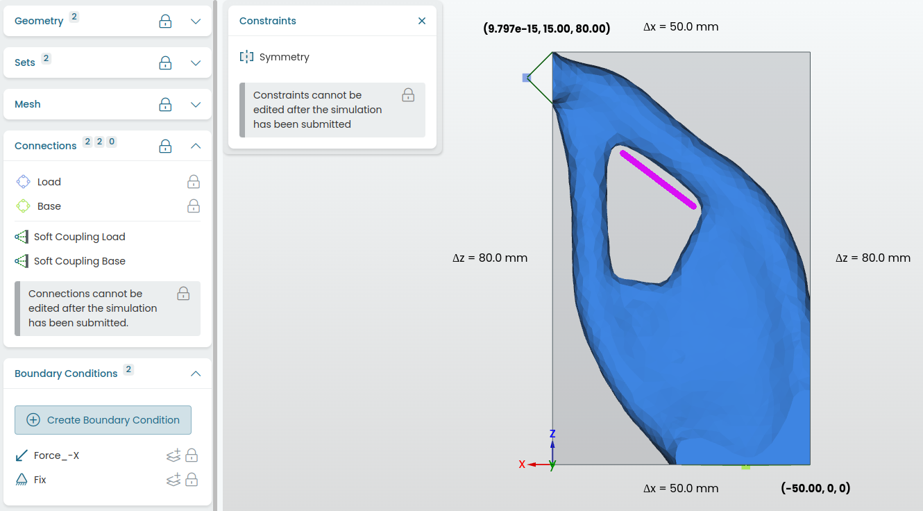
Fig. 13.8 Optimized shape with marked overhang region

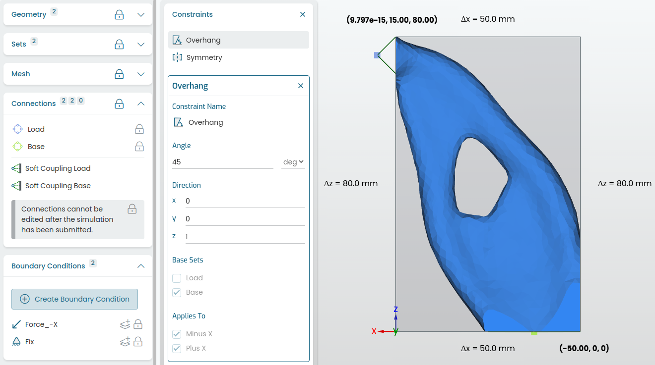
Fig. 13.9 Optimized shape with overhang angle set to 45°

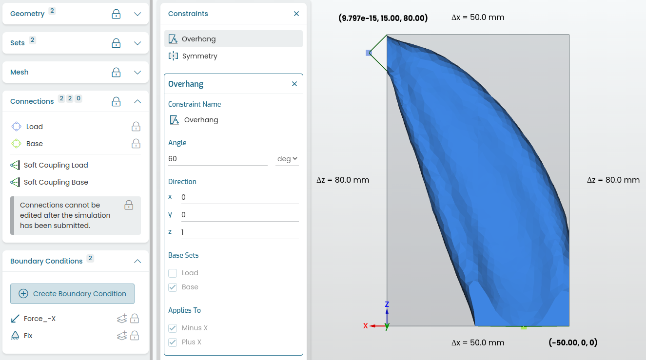
Fig. 13.10 Optimized shape with overhang angle set to 60°

13.2.5.2. Base Sets

When the design space features unavoidable overhangs, it is necessary to include any additionally supported sets in the selection of base sets.

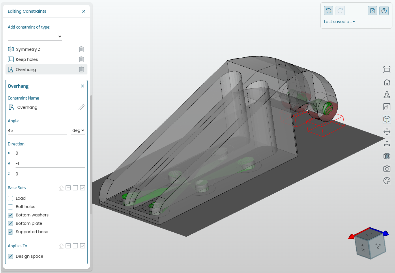
Fig. 13.11 Example of a design space with unavoidable overhang: red boxes mark expected positioning of additional supports

Tip

The combination of the main optimization constraints presented above can produce complex designs for thin wall castings, ribs, additive manufacturing and injection molding applications.

13.2.6. Combining Constraints

The following project examples and tutorials show how a combination of main constraints and model setups can be used to achieve different manufacturing objectives in Möbius.

This section only includes a brief outline of capabilities and examples. For more details to your specific optimization project, please contact Rafinex (support@rafinex.com).

13.2.6.1. Celanese Engine Bracket

Fig. 13.12 shows an example for an injection molding application of an engine bracket performed in conjunction with the Celanese R&D center in Geneva.

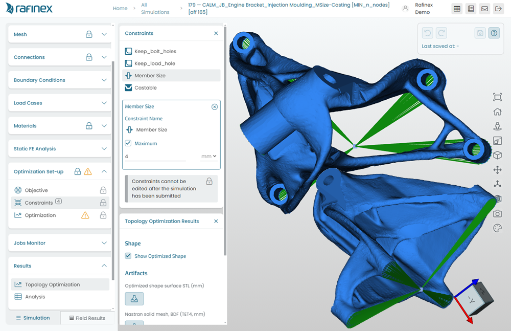
Fig. 13.12 Celanese engine bracket

Note

Public references for the above optimization project with Celanese can be found through the following links:

• Rafinex & Celanese article (1)

• Rafinex & Celanese article (2)

The Möbius optimized design achieved a mass reduction of 25%, while increasing its stiffness by 30% (lower total strain energy) over the production bracket.

Fig. 13.13 shows a comparison of the Rafinex optimized design (blue) vs the production design.

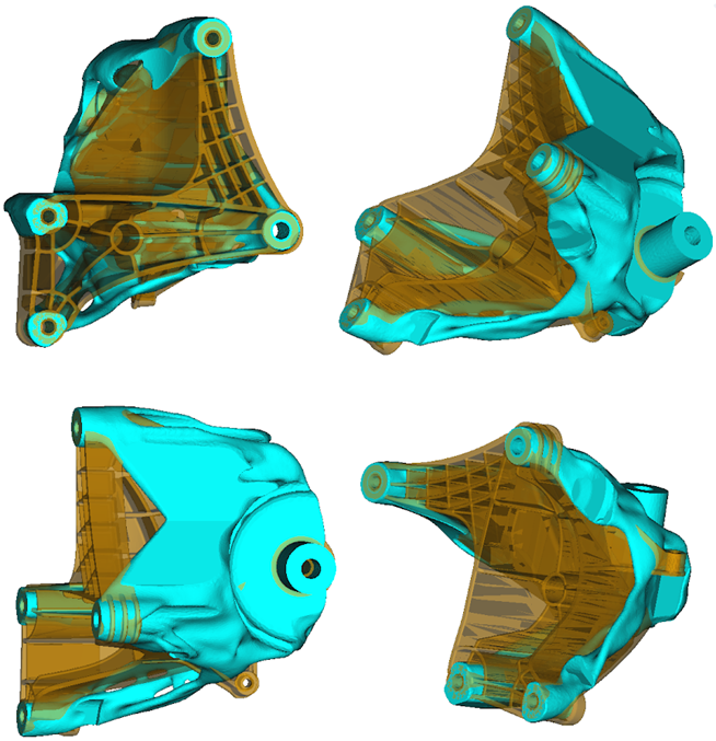
Fig. 13.13 Production vs Rafinex engine bracket

13.2.6.2. Robot Gripper (Hollow)

Fig. 13.14 shows an example of a 3D printed hollow robot gripper.

Fig. 13.14 Robot gripper

Note

Public references for the above robot gripper optimization project can be found through the following links:

• Rafinex robot gripper video - short (1)

• Rafinex robot gripper video - full (2)

The Möbius optimized design achieved a mass reduction of 51%, while keeping its stiffness and reduced stress levels over the production gripper.

13.2.6.3. ECU Bracket (3 variants)

This tutorial shows how an Electronics Control Unit (ECU) bracket was optimized via three different approaches.

Fig. 13.15 shows an example of light-weighting a Baseline plate design.

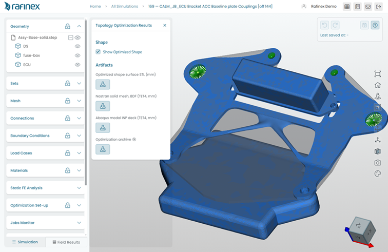
Fig. 13.15 ECU bracket - Baseline

Fig. 13.16 shows an example of a similar setup where the design space was extended (into a square plate) to improve the final design.

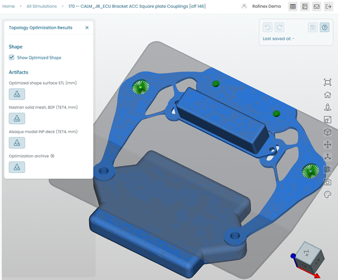
Fig. 13.16 ECU bracket - Plate

Fig. 13.17 shows an example of a 3D printed version for maximum strength.

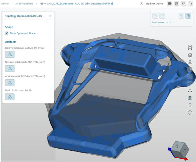
Fig. 13.17 ECU bracket - 3D print

13.2.6.4. Radar Assembly

This tutorial shows an application of topology optimization on a large structural assembly. This model features two sub-assemblies (azimuth & elevation) with their corresponding bearings and torsional stiffness for each drive unit (motor).

Fig. 13.18 shows an example of light weighting a Baseline large design.

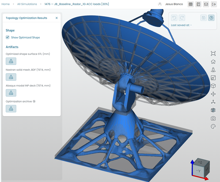
Fig. 13.18 Baseline radar assembly

Fig. 13.19 shows an example of optimizing the complete assembly design via increasing the design space (packaging space) available.

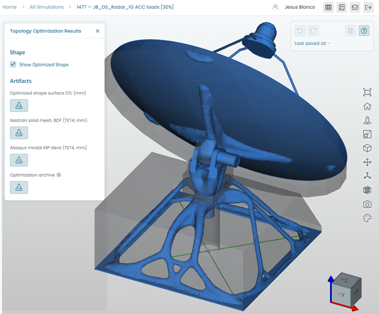
Fig. 13.19 Design Space radar assembly

Fig. 13.20 shows a typical application in Möbius for a complex assembly with the total strain energy (TSE) breakdown on a per part (volume) and load case basis.

These outputs help to decide what areas of the assembly matter for structural optimization, and main contributions to the overall stiffness of the assembly. Furthermore, the worst load cases (highest TSE) of interest can be easily identified at a glance.

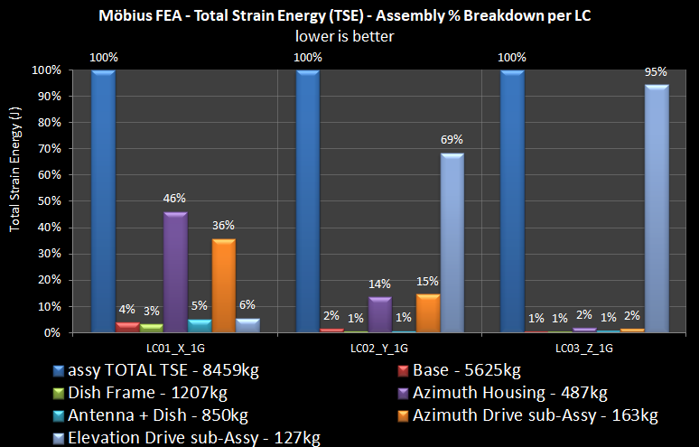
Fig. 13.20 Total Strain Energies - radar assembly

13.2.6.5. Suspension Control Arm (3 variants)

This tutorial shows how a vehicle suspension control arm was optimized for three different manufacturing approaches.

Fig. 13.21 shows an example of a 3D printed variant.

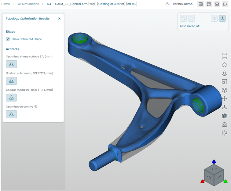
Fig. 13.21 Suspension arm - 3d print

Fig. 13.22 shows an example of a hollow casting variant with a split middle wall.

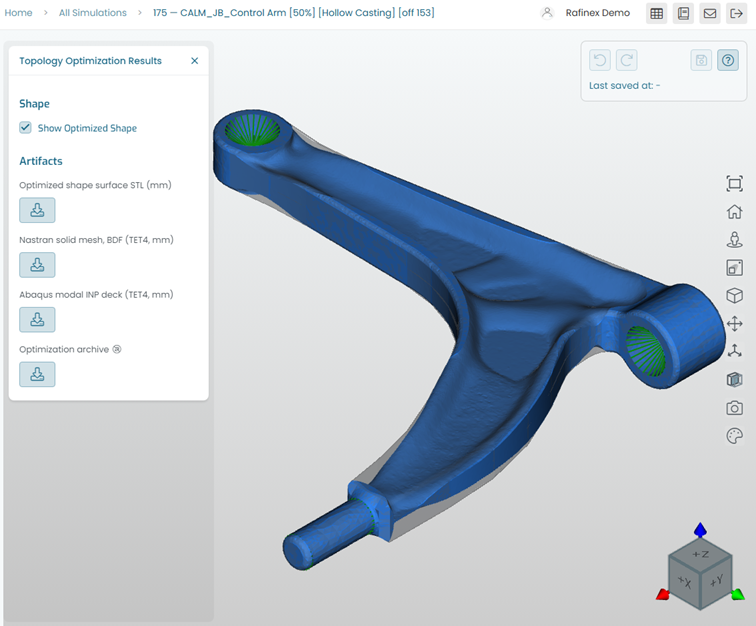
Fig. 13.22 Suspension arm - hollow casting

Fig. 13.23 shows an example of a hollow 3D print variant for maximum stiffness while light weighting.

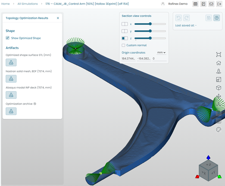
Fig. 13.23 Suspension arm - hollow 3D print

13.2.6.6. Aerospace Hinge (2 variants)

This tutorial shows how an aerospace hinge bracket was optimized for different manufacturing approaches.

Fig. 13.24 shows an example of a 3D printed variant.

Fig. 13.24 Aerospace hinge - 3D print

Fig. 13.25 shows an example of a casting manufacturing constraint variant.

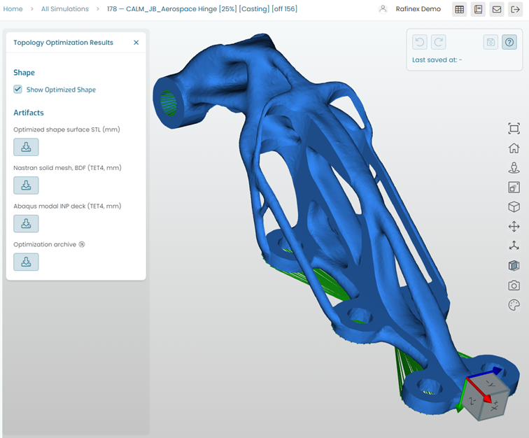
Fig. 13.25 Aerospace hinge - casting

13.2.6.7. Car (load paths)

This tutorial shows how a vehicle initial concept envelope can be studied with 10 load cases to reveal complex load paths for stiffness.

Fig. 13.26 shows an example of a load paths optimization study.

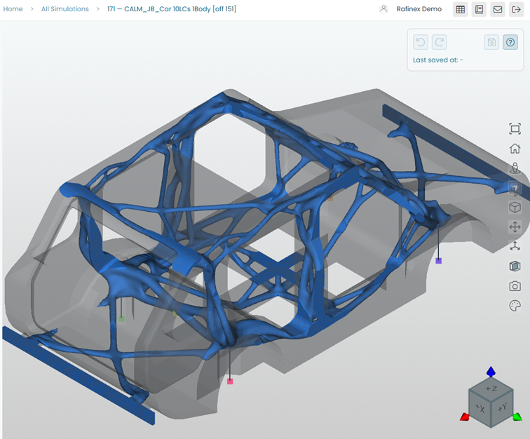
Fig. 13.26 Car 10 load cases - load paths

13.2.6.8. Motor Bracket

This tutorial shows how a motor bracket can be studied with 10 load cases to reveal complex load paths for stiffness and 3D printing.

Fig. 13.27 shows an example of a load paths optimization study.

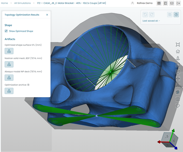
Fig. 13.27 Motor bracket 10 load cases

Tip

All the tutorial and public project models presented in this section can be made available to all Möbius users. Please contact Rafinex (support@rafinex.com) for more details.

13.3. Optimization

The Optimization panel allows selecting load cases and optimization options, and submitting the analysis into the cloud solving environment.

It is recommended to leave the solver and refine settings as per defaults at the start of a new model or project. It is rare that non-default settings are required. This will depend on the complexity of the model setup and objectives.

Fig. 13.28 shows this panel.

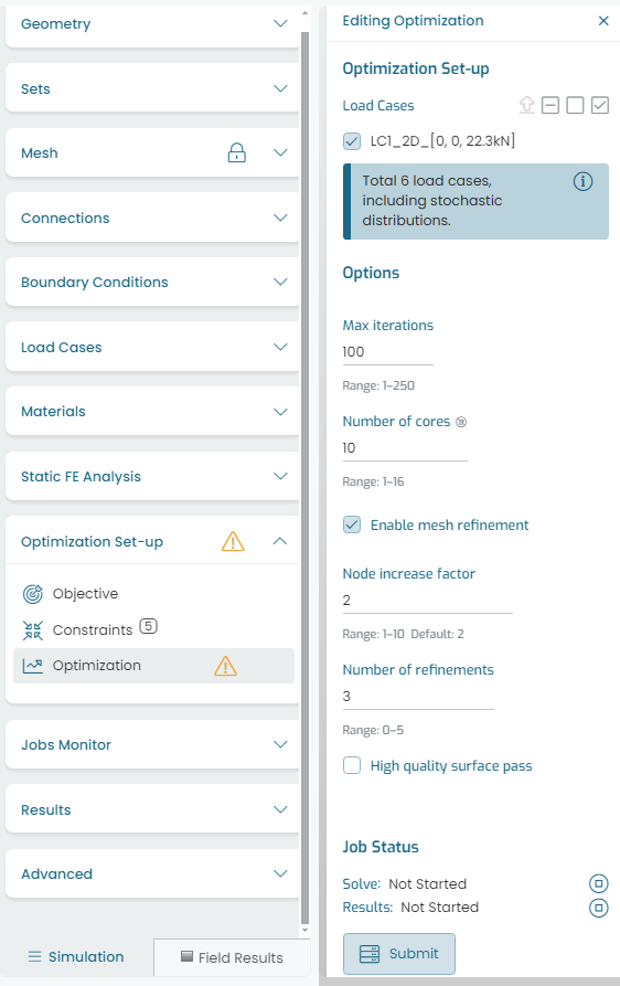
Fig. 13.28 Optimization setup and solve