10. Boundary Conditions
In this panel users can apply constraints and loads to the model setup via sets. Each boundary condition entry features a clone and delete button. The clone button makes duplicates for fast generation of loads and constraints.
The same logic as per Geometry and Sets panels applies: clicking on an item will open the editing panel.
10.1. Constraints
Arguably, the most important part of setting a structural linear statics model up, is to apply correct constraints to represent reality as close as possible.
The following figure shows the Fixed condition under the drop-down menu. Depending on whether the constraint is applied to a surface set (not recommended) or a coupling reference node (recommended), the degrees of freedom (DOF) available will be 3 (3 translations) or 6 (3 translations and 3 rotations) respectively.
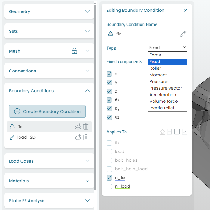
Fig. 10.1 Applying constraints
Fig. 10.1 also shows how coupling reference points are highlighted with the same color as they appear in the display area and in the Connections panel list.
Tip
It is highly recommended to avoid constraining a surface set, as this will result in an over-constrained local area. This situation does not exist in reality in typical structures. Everything moves ever so slightly with respect to different locations. Even if it is only a few micron, depending on the setup, it can produce an unrealistically high local stiffness area.
A more realistic way to constrain a model is at reference points on Soft (preferred) couplings. These allow for small local compliance, which tends to yield more realistic results.
Note
The Roller condition shown in figure above is for legacy purposes, and should not be used.
The correct way to model a roller condition is to build a soft coupling, and constrain its reference point accordingly, typically leaving one rotation DOF free.
10.2. Force Vector
Fig. 10.2 shows the Force vector load application. A force vector can be applied to a surface set or a coupling reference point (recommended).
The main advantage of applying a force vector on a coupling node is that it will produce the corresponding moments contribution from the geometry and location of the reference point with respect to the coupling surface set.
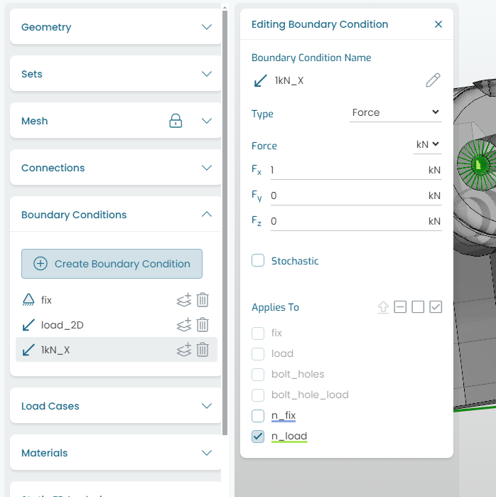
Fig. 10.2 Applying loads: force vector
10.2.1. Stochastic (Force vector) Distributions
The stochastic (force) distribution perturbs the nominal force direction, rotating the vector while keeping the magnitude constant. This essentially generates additional loads over a 2D plane or a 3D cone distribution.
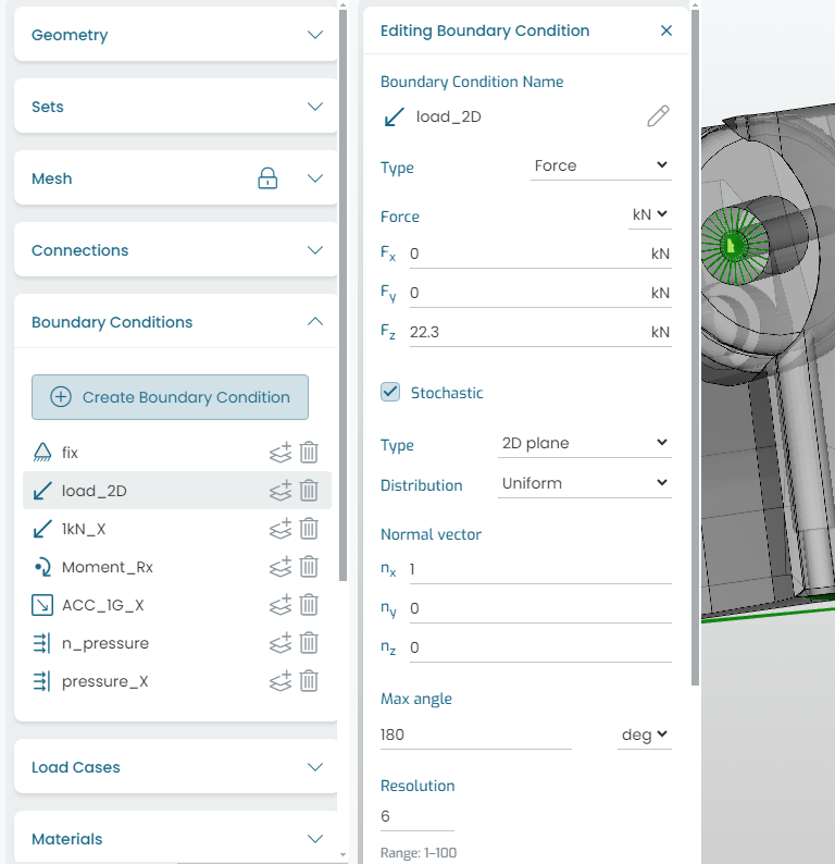
Fig. 10.3 Applying stochastic loads: 2D force vector distribution
Note
Care should be taken when applying stochastic loads. Vector samples requested represent additional load cases in the optimization analysis, with the consequent additional solving time.
Furthermore, if a structural FEA setup already produces complex loadpaths with realistic combinations of bending and torsional moments, it is likely that stochastic perturbations with small angles will produce hardly any difference in the results. This is due to pure physics from the nominal setup.
It is also noted that when performing an FEA validation analysis with stochastic loads, the results generated will be of statistical nature, and possibly hard to compare directly to previous validations with nominal loads. Users must plan how to model and post-process results that make sense for their specific structural project.
Tip
An extensive explanation and several examples of Möbius stochastics implementation for 2D and 3D distributions can be found in the Pylon Benchmark section.
10.3. Moment Vector
Fig. 10.4 shows the Moment vector load application. A moment vector can be applied to a surface set or a coupling reference point (recommended).
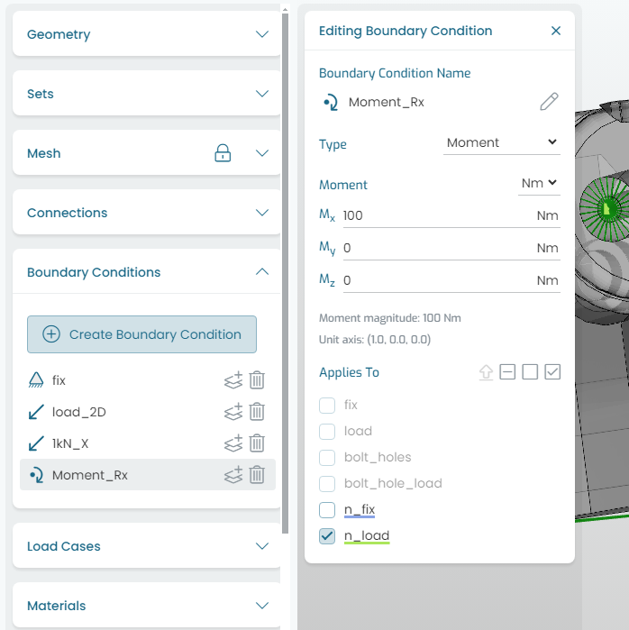
Fig. 10.4 Applying loads: moment vector
Note
The effects of moments on a structure should not be underestimated. It is the addition of bending and torsional moments effects that typically causes a structure to reach its stress or stiffness limits.
10.4. Acceleration
Fig. 10.5 shows the Acceleration vector load application. An acceleration vector can be applied to a volume (solid part).
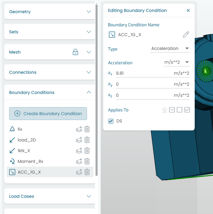
Fig. 10.5 Applying loads: acceleration vector
Note
It is common practice at design concept stage, to check an assembly via 3 unit acceleration load cases; e.g. 1G in each direction. These type of unit loads give an initial set of results that help to understand main load paths quickly.
Furthermore, for assemblies, it produces total strain energy levels per part, which can be used to rank critical parts in an assembly to be first optimized.
Acceleration loads are applied in a quasi-static manner. Further checks with the optimized assembly model should be performed for linear dynamics.
10.5. Normal Pressure
Fig. 10.6 shows the (normal) Pressure vector load application. A normal pressure can be applied to surface sets.
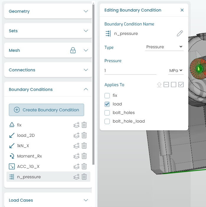
Fig. 10.6 Applying loads: normal pressure
Tip
When applying a normal pressure on complex geometry, it is of interest to calculate the total force vector produced by this loading input. This can be easily checked by solving a preliminary FEA of the setup, and inspecting the sum of all reaction forces and moments in the output text results file (CSV).
10.6. Pressure Vector
Fig. 10.7 shows the Pressure vector load application. A pressure vector can be applied to surface sets.
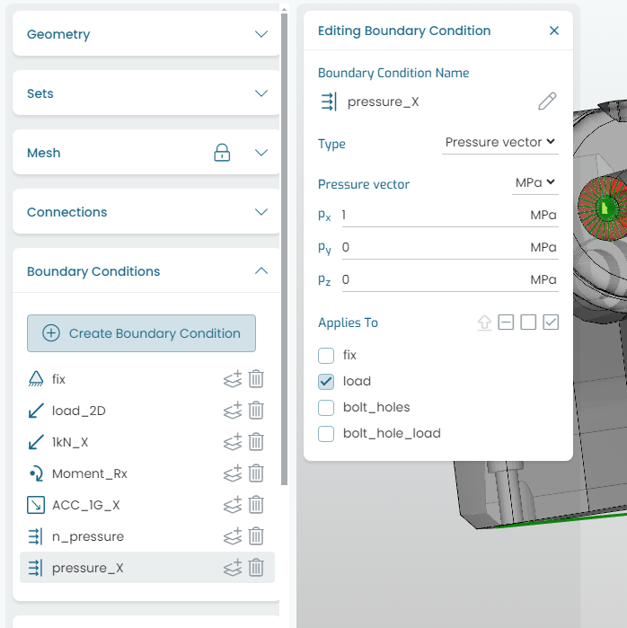
Fig. 10.7 Applying loads: pressure vector