Beams 

Beam theory provides a framework for modeling the behavior of slender solids—structures with longitudinal dimensions significantly larger than their cross-sectional dimensions—under complex loading conditions. By mathematically collapsing the 3D volume onto a representative centerline, this framework reduces the structural analysis of beams to a computationally efficient 1D model.

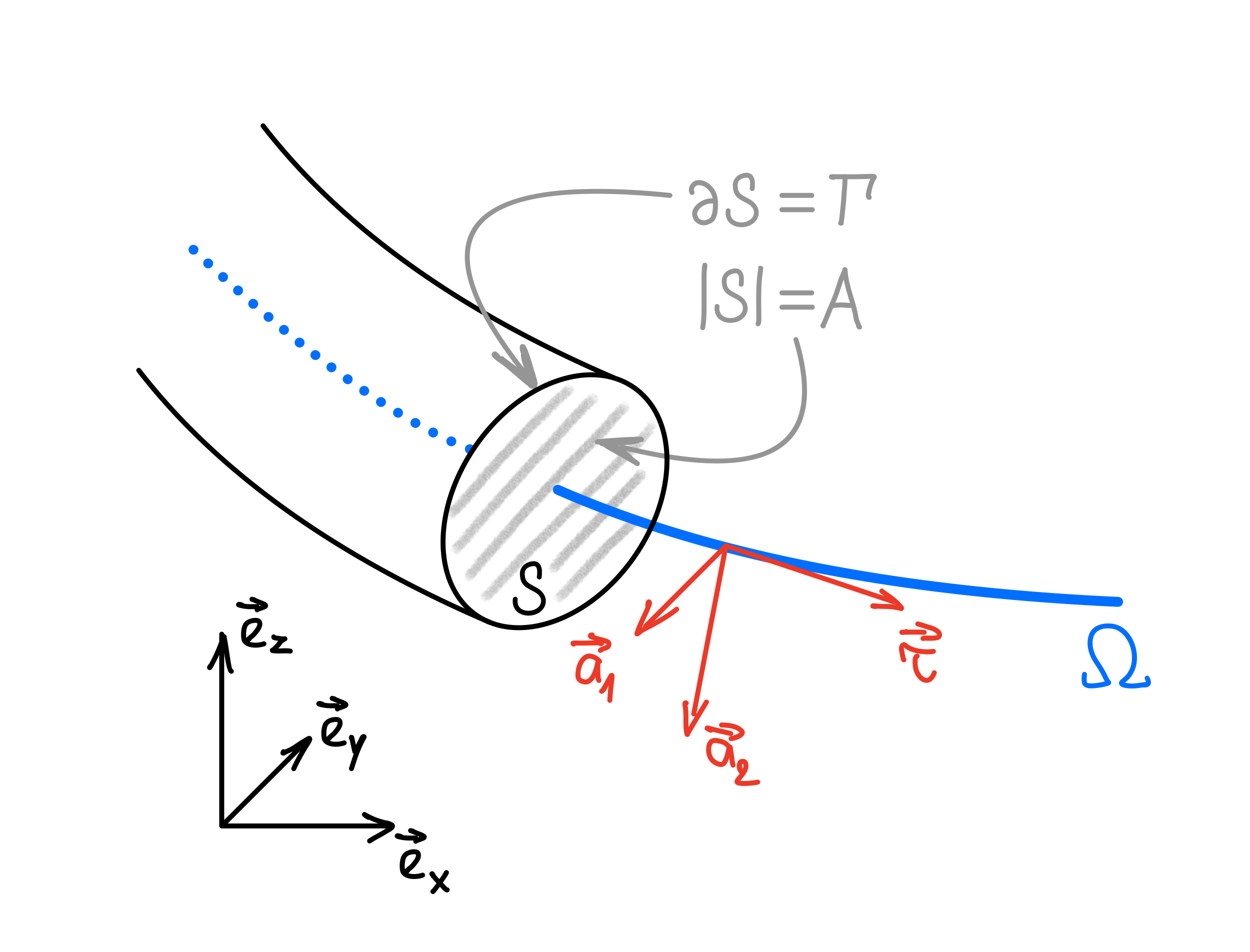
Reduced beam model — Fig. 15 Illustration of the reduced beam model with the cross-section \(S\), computational domain \(\Omega\), and local coordinate frame \(\{\vtau, \va_1, \va_2\}\).

Möbius implements the beam model with the following characteristics:

This documentation provides a rigorous derivation of the governing equations for the beam model based on the aforementioned assumptions, and a comprehensive guide to the load cases and deformations supported by the current framework. It outlines key implementation caveats, ensuring a transparent understanding of the model’s application range and current limitations.

Introduction 

While the general implementation is based on introducing a local coordinate frame for each linear segment of the beam geometry, see Fig. 15, we will first analyze a beam in a simplified configuration.

In particular, we take a prismatic beam of length \(L\) and cross-section \(S\) of area \(A\), we align its longitudinal axis with the \(x\) axis, and we orient \(y\) and \(z\) axes to match the principal axes of inertia of the cross-section. The computational domain is in this case given by \(\Omega = (0, L) \subset \R\) with its boundary consisting of the discrete endpoints \(\partial\Omega = \{0, L\}\).

Classical beam theories—including both Euler-Bernoulli and Timoshenko-Ehrenfest models—assume that plane cross-sections remain plane after deformation. This unlocks the possibility to describe the state of the beam in terms of cross-sectional displacements and rotations, rather than tracking every individual point in the 3D volume.

Another key assumption says that the lateral surface of the beam remains stress-free. To satisfy this no-traction boundary condition for general (non-circular) cross-sections, the “plane sections remain plane” constraint must be relaxed in favor of a warping-corrected axial displacement allowing for an out-of-plane deformation in torsion.

These considerations lead to the kinematic ansatz

\begin{align} \vu^{\mathrm{3D}}(x, y, z) &= \begin{bmatrix} u_x(x) + z \theta_y(x) - y \theta_z(x) + \psi(y, z) \eta(x) \\ u_y(x) - (z - z_s) \theta_x(x) \\ u_z(x) + (y - y_s) \theta_x(x) \end{bmatrix}, \end{align}

where \(\vu = [u_x, u_y, u_z]^T\) and \(\vtheta = [\theta_x, \theta_y, \theta_z]^T\) denote cross-sectional displacements and rotations respectively, \(\eta\) is a warping parameter, and \(\psi\) is a torsional warping function given by the geometry of the cross-section. Last but not least, the point \((y_s, z_s)\) represents the shear center of the cross-section.

The above expression can be rewritten in a compact vector form

\begin{align} \vu^{\mathrm{3D}}(\vx) &= \vu(x) + \vtheta(x) \times \vX - \theta_x(x) \ve_x \times \vX_s + \eta(x) \psi(\vX) \ve_x, \end{align}

where \(\vx = x \ve_x + \vX\) is a point in the 3D volume, \(\vX = [0, y, z]^T\) is its in-section position vector, while \(\vX_s = [0, y_s, z_s]^T\) is the in-section position vector of the shear center. In what follows, we use prime \(()'\) to denote the derivative with respect to \(x\).

Note

The torsional warping function is obtained by solving a boundary value problem corresponding to the static equilibrium equation with the no-traction boundary condition in the Saint-Venant approximation of pure torsion, see e.g. [Pilkey, 2002].

The following observations can be made based on the parametrization of the displacement field by the triplet \((\vu, \vtheta, \eta)\):

The longitudinal displacement arises from bending rotations about the centroid, its axial translation, and out-of-plane distortion due to torsional warping.
The transverse displacements are defined by torsional rotation about the shear center and its lateral deflections.

These kinematic assumptions can be applied to derive beam models within the Vlasov theory, where the warping parameter \(\eta\) governs the rate of non-uniform warping, see e.g. [Back and Will, 1998]. The model presented here adheres to a simplified framework by employing the Saint-Venant torsion theory, which identifies \(\eta\) as \(\theta_x'\), and thereby leads to the parametrization of the displacement by 6 degrees of freedom \((u_x, u_y, u_z, \theta_x, \theta_y, \theta_z)\).

Table 1 outlines selected cross-sectional properties used throughout the documentation.

Table 1 Cross-sectional properties
Definition	Name	Unit
\(A = \int_S \d{S}\)	cross-sectional area	\(\mathrm{m^2}\)
\(I_y = \int_S z^2 \d{S}\)	area moment of inertia about \(y\)-axis	\(\mathrm{m^4}\)
\(I_z = \int_S y^2 \d{S}\)	area moment of inertia about \(z\)-axis	\(\mathrm{m^4}\)
\(J = \int_S [(z - z_s - \partial_y \psi)^2 + (y - y_s + \partial_z \psi)^2]\d{S}\)	torsional constant	\(\mathrm{m^4}\)

Theoretical framework 

The cornerstone of engineering beam theory is the assumption that the longitudinal normal stress \(\sigma_{xx}\) is the primary structural response, while \(\sigma_{yy}\) and \(\sigma_{zz}\) can be neglected (orders of magnitude smaller in slender structures). This reduction is endorsed by the no-traction boundary condition on the lateral surface, which constrains the development of transverse stress fields.

Linear elasticity 

A simple algebraic manipulation can be used to invert the stress-strain constitutive relation for isotropic, linear elastic materials. The diagonal components of the strain tensor satisfy

\begin{align} \epsilon_{xx} &= \frac{1}{E} \left[ \sigma_{xx} - \nu (\sigma_{yy} + \sigma_{zz}) \right], \\ \epsilon_{yy} &= \frac{1}{E} \left[ \sigma_{yy} - \nu (\sigma_{xx} + \sigma_{zz}) \right], \\ \epsilon_{zz} &= \frac{1}{E} \left[ \sigma_{zz} - \nu (\sigma_{xx} + \sigma_{yy}) \right], \end{align}

while the off-diagonal components obey the simple relations

\begin{align} \epsilon_{xy} &= \frac{1}{2G} \sigma_{xy}, & \epsilon_{xz} &= \frac{1}{2G} \sigma_{xz}, & \epsilon_{yz} &= \frac{1}{2G} \sigma_{yz}, \end{align}

where \(G = \frac{1}{2} E (1 + \nu)^{-1}\) denotes the shear modulus.

By considering \(\sigma_{yy} = \sigma_{zz} = 0\), we allow the beam to stretch/shrink in transverse directions freely. This fundamental assumption leads to the following simple relations:

the Hooke law in the axial direction

\begin{align} \sigma_{xx} = E \epsilon_{xx}, \end{align}

the Poisson effect in the transverse directions

\begin{align} \epsilon_{yy} = \epsilon_{zz} = -\nu \epsilon_{xx}. \end{align}

Note that the second expression clearly contradicts the above kinematic ansatz which assumes rigid cross-sections (\(\epsilon_{yy} = \epsilon_{zz} = 0\)).

Classical beam theories neglect the lateral deformation due to the Poisson effect, assuming it does not affect the bending behavior significantly. In other words, the strain energy contribution arising due to the Poisson effect is assumed negligible.

The Saint-Venant torsion theory assumes \(\eta = \theta_x'\) and uniform warping, i.e. \(\eta' = 0\). It thus neglects the strain energy contribution associated with non-uniform warping.

Based on the accepted kinematic ansatz, we write the strain tensor \(\teps = \frac{1}{2} \left(\nabla \vu + \nabla \vu^T \right)\) in the matrix form

\begin{align} \teps &= \begin{bmatrix} \epsilon_{xx} & \frac{1}{2} \gamma_{xy} & \frac{1}{2} \gamma_{xz} \\ \frac{1}{2} \gamma_{xy} & 0 & 0 \\ \frac{1}{2} \gamma_{xz} & 0 & 0 \end{bmatrix}, \end{align}

where

\begin{align} \epsilon_{xx} &= u_x' + z \theta_y' - y \theta_z', \\ \gamma_{xy} &= u_y' - \theta_z - (z - z_s - \partial_y \psi) \theta_x', \\ \gamma_{xz} &= u_z' + \theta_y + (y - y_s + \partial_z \psi) \theta_x'. \end{align}

By introducing the strain vector \(\veps = [\epsilon_{xx}, \gamma_{xy}, \gamma_{xz}]^T\), along with the cross-sectional strains

\begin{align} \vgamma &= \vu' + \ve_x \times \vtheta, & \vomega &= \vtheta', \end{align}

see Table 2, it is possible to write the above relations in a compact vector form

\begin{align} \veps &= \vgamma + \vomega \times \vX - (\ve_x \times \vX_s - \nabla \psi) (\vomega \cdot \ve_x). \end{align}

Finally, the stress tensor takes the matrix form

\begin{align} \tsigma &= \begin{bmatrix} \sigma_{xx} & \sigma_{xy} & \sigma_{xz} \\ \sigma_{xy} & 0 & 0 \\ \sigma_{xz} & 0 & 0 \end{bmatrix}, \end{align}

with the non-vanishing components satisfying the constitutive relations

\begin{align} \sigma_{xx} &= E \epsilon_{xx}, & \sigma_{xy} &= G \gamma_{xy}, & \sigma_{xz} &= G \gamma_{xz}. \end{align}

These components can be collected in the stress vector \(\vsigma = [\sigma_{xx}, \sigma_{xy}, \sigma_{xz}]^T\) and used to define the internal forces and moments

\begin{align} \vF &= \int_S \vsigma \d{S}, & \vM &= \int_S \left[ \vX \times \vsigma - (\vX_s \times \vsigma) \cdot \ve_x + (\vsigma \cdot \nabla \psi) \ve_x \right], \end{align}

see Table 2.

Table 2 Cross-sectional strains, internal forces and moments
Definition	Name	Unit	Definition	Name	Unit
\(\gamma_x = u_x'\)	normal strain	\(-\)	\(F_x = \int_S \sigma_{xx} \d{S}\)	normal force	\(\mathrm{N}\)
\(\begin{align} \gamma_y &= u_y' - \theta_z \\ \gamma_z &= u_z' + \theta_y \end{align}\)	shear strains	\(-\)	\(\begin{align} F_y &= \textstyle{\int_S \sigma_{xy} \d{S}} \\ F_z &= \textstyle{\int_S \sigma_{xz} \d{S}}\end{align}\)	shear forces	\(\mathrm{N}\)
\(\omega_x = \theta_x'\)	torsional strain	\(\mathrm{m^{-1}}\)	\(\begin{align} M_x &= \textstyle{\int_S[(y - y_s + \partial_z \psi)\sigma_{xz}} \\ &\ \ \textstyle{-(z - z_s - \partial_y \psi)\sigma_{xy}]\d{S}}\end{align}\)	torsional moment	\(\mathrm{Nm}\)
\(\begin{align} \omega_y &= \theta_y' \\ \omega_z &= \theta_z' \end{align}\)	bending curvatures	\(\mathrm{m^{-1}}\)	\(\begin{align} M_y &= \textstyle{\int_S z\sigma_{xx} \d{S}} \\ M_z &= \textstyle{-\int_S y\sigma_{xx} \d{S}} \end{align}\)	bending moments	\(\mathrm{Nm}\)

Strain energy 

The internal strain energy is given by

\begin{align} U &= \frac{1}{2} \int_\Omega \int_S \tsigma : \teps \d{S} \d{x}. \end{align}

Given the above simplifications, the integrand naturally splits into axial and shear components

\begin{align} U &= \frac{1}{2} \int_\Omega \int_S \left( \sigma_{xx} \epsilon_{xx} + \sigma_{xy} \gamma_{xy} + \sigma_{xz} \gamma_{xz} \right) \d{S} \d{x}. \end{align}

At this point, it is possible to proceed in two ways. First, using the definitions from Table 2, we see that

\begin{align} U &= \frac{1}{2} \int_\Omega \left( F_x \gamma_x + F_y \gamma_y + F_z \gamma_z + M_x \omega_x + M_y \omega_y + M_z \omega_z \right) \d{x}. \end{align}

On the other hand, when we first substitute for the stress components from the linear elasticity constitutive relations and then we integrate over \(S\), we obtain

\begin{align} U &= \frac{1}{2} \int_\Omega \left[ E A \gamma_x^2 + G A_y \gamma_y^2 + G A_z \gamma_z^2 + G J \omega_x^2 + E I_y \omega_y^2 + E I_z \omega_z^2 \right] \d{x}. \end{align}

Here, we introduced the effective shear areas, \(A_y = \kappa_y A\) and \(A_z = \kappa_z A\), with the shear deformation coefficients \(\kappa_y\) and \(\kappa_z\). These coefficients scale the strain energy stored in the reduced 1D model (with uniform shear stresses) to match the strain energy in the full 3D model (with non-uniform shear stresses), see e.g. [Pilkey, 2002].

Note

Each shear deformation coefficient can be computed by solving a boundary value problem for the shear warping function (not introduced in our kinematic ansatz). In contrast to torsional warping, the Poisson ratio \(\nu\) enters the governing equations and makes the coefficients dependent not only on the geometry, but also on the material properties.

By comparing the last two expressions for the strain energy \(U\), we derive the cross-sectional stress-strain relations

\begin{align} \begin{bmatrix} F_x \\ F_y \\ F_z \\ M_x \\ M_y \\ M_z \end{bmatrix} &= \begin{bmatrix} E A & & & & & \\ & G A_y & & & & \\ & & G A_z & & & \\ & & & G J & & \\ & & & & E I_y & \\ & & & & & E I_z \end{bmatrix} \begin{bmatrix} \gamma_x \\ \gamma_y \\ \gamma_z \\ \omega_x \\ \omega_y \\ \omega_z \end{bmatrix}. \end{align}

Stress distribution 

To get an approximate stress distribution across the beam, we invert the above equation and substitute the result back to the linear elasticity constitutive relations.

The normal stress resulting from an axial force \(F_x\) and bending moments \(M_y\) and \(M_z\) is given by

\begin{align} \sigma_{xx}(x, y, z) &= \frac{F_x(x)}{A} - \frac{M_z(x)}{I_z} y + \frac{M_y(x)}{I_y} z. \end{align}

The shear stresses resulting from a torsional moment \(M_x\) are given by

\begin{align} \sigma_{xy}^\mathrm{tor}(x, y, z) &= \frac{M_x(x)}{J}\left[ \partial_y \psi(y, z) - (z - z_s) \right], \\ \sigma_{xz}^\mathrm{tor}(x, y, z) &= \frac{M_x(x)}{J}\left[ \partial_z \psi(y, z) + (y - y_s) \right]. \end{align}

The shear stresses resulting from transverse shear forces \(F_y\) and \(F_z\) are given by

\begin{align} \sigma_{xy}^\mathrm{flex}(x, y, z) &= \frac{F_y(x)}{A_y}, \\ \sigma_{xz}^\mathrm{flex}(x, y, z) &= \frac{F_z(x)}{A_z}. \end{align}

Note

The formulas for the flexural shear stresses provide a rough approximation of the real stress distribution, which is not constant across the cross-section. As such, these expressions are not suitable for estimating the peak stress values. For that specific purpose, it is recommended to use formulas based on the shear warping functions, see e.g. [Pilkey, 2002].

The total shear stresses are given by

\begin{align} \sigma_{xy} &= \sigma_{xy}^\mathrm{tor} + \sigma_{xy}^\mathrm{flex}, \\ \sigma_{xz} &= \sigma_{xz}^\mathrm{tor} + \sigma_{xz}^\mathrm{flex}. \end{align}

Finally, the von Mises stress is obtained as

\begin{align} \sigma_{\mathrm{vM}} &= \sqrt{\sigma_{xx}^2 + 3(\sigma_{xy}^2 + \sigma_{xz}^2)}. \end{align}

External loads 

To establish a rigorous energy balance for the beam model, we categorize the external loading into three distinct physical sources based on their domain of application, see Table 3. This distinction is fundamental to the variational derivation, as it ensures that the work done by volumetric body forces, lateral surface tractions, and end-face tractions is consistently mapped to the 1D generalized resultants, see Table 4.

Table 3 External loads in 3D
Symbol	Name	Unit	Domain
\(\vf\)	volumetric body force	\(\mathrm{N/m^3}\)	\(\Omega \times S\)
\(\vg\)	lateral surface traction	\(\mathrm{N/m^2}\)	\(\Omega \times \Gamma\), where \(\Gamma \equiv \partial S\)
\(\vt\)	end-face traction	\(\mathrm{N/m^2}\)	\(\partial\Omega \times S\)

Table 4 External loads in 1D
Definition	Name	Unit	Domain
\(\vf^d = \int_S \vf \d{S} + \int_\Gamma \vg \d{\Gamma}\)	distributed force	\(\mathrm{N/m}\)	\(\Omega\)
\(\begin{align}\vm^d &= \textstyle{\int_S \vX \times \vf \d{S}} \\ &\quad \textstyle{+\int_\Gamma \vX \times \vg\ \d{\Gamma} - [(\vX_s \times \vf^d) \cdot \ve_x] \ve_x}\end{align}\)	distributed moment	\(\mathrm{N m/m}\)	\(\Omega\)
\(b_\omega^d = \int_S \psi f_x \d{S}\ + \int_\Gamma \psi g_x \d{\Gamma}\)	distributed bimoment	\(\mathrm{N m^2/m}\)	\(\Omega\)
\(\vF^c = \int_S \vt \d{S}\)	concentrated force	\(\mathrm{N}\)	\(\partial\Omega\)
\(\vM^c = \int_S \vX \times \vt \d{S}\ - [(\vX_s \times \vF^c) \cdot \ve_x] \ve_x\)	concentrated moment	\(\mathrm{N m}\)	\(\partial\Omega\)
\(B_\omega^c = \int_S \psi t_x \d{S}\)	concentrated bimoment	\(\mathrm{N m^2}\)	\(\partial\Omega\)

Important

The current formulation assumes warping-neutral loading. This means that external loads are distributed in a way that bimoments remain zero, i.e.

\begin{align} b_\omega^d = B_\omega^c = 0, \end{align}

so that the longitudinal forces do not induce torsional deformation.

Variational problem 

We derive the static equilibrium equations for the proposed beam model by minimizing the potential energy

\begin{align} \Pi &= U - W_{\mathrm{ext}}, \end{align}

where the external work is given by

\begin{align} W_{\mathrm{ext}} &= \int_\Omega \left( \int_S \vf \cdot \vu^{\mathrm{3D}} \d{S} + \int_\Gamma \vg \cdot \vu^{\mathrm{3D}} \d{\Gamma} \right) \d{x} + \int_{\partial\Omega} \int_S \vt \cdot \vu^{\mathrm{3D}} \d{S} \d{P} \\ &= \int_\Omega \left( \vf^d \cdot \vu + \vm^d \cdot \vtheta \right) \d{x} + \int_{\partial\Omega} \left( \vF^c \cdot \vu + \vM^c \cdot \vtheta \right) \d{P} \end{align}

The use of the point measure \(\d{P}\) over the boundary \(\partial\Omega\) allows for the integration of discrete resultants, effectively recovering the concentrated forces and moments acting at the endpoints. The resulting variational equation reads

\begin{align} &\int_\Omega \left( \vF \cdot \delta{\vgamma} - \vf^d \cdot \delta{\vu} + \vM \cdot \delta{\vomega} - \vm^d \cdot \delta{\vtheta} \right) \d{x} - \int_{\partial\Omega}\left( \vF^c \cdot \delta{\vu} + \vM^c \cdot \delta{\vtheta} \right)\d{P} = 0. \end{align}

Given the definitions in Table 2, we rearrange the terms in the first integral, so it becomes

\begin{align} &\int_\Omega \left( \vF \cdot \delta{\vu'} - (\ve_x \times \vF) \cdot \delta{\vtheta} - \vf^d \cdot \delta{\vu} + \vM \cdot \delta{\vtheta'} - \vm^d \cdot \delta{\vtheta} \right) \d{x}. \end{align}

Integrating by parts, we can formally identify the beam model as a boundary value problem with the governing equations

\[\begin{split}\left. \begin{aligned} -\vF' &= \vf^d \\ -\vM' - \ve_x \times \vF &= \vm^d \end{aligned} \quad \right\} \quad \forall x \in \Omega = (0, L),\end{split}\]

subjected to a suitable combination of Neumann and Dirichlet boundary conditions

\[\begin{split}\left. \begin{aligned} n_x \vF &= \vF^c &\mathrm{or}\qquad \vu &= \vu^c \\ n_x \vM &= \vM^c &\mathrm{or}\qquad \vtheta &= \vtheta^c \end{aligned} \quad \right\} \quad \forall x \in \partial \Omega = \{0, L\},\end{split}\]

where \(n_x\) denotes the component of the outward unit normal vector to the beam surface, so that \(n_x|_{x=0} = -1\) and \(n_x|_{x=L} = 1\).

Implementation 

Beam models implemented in Möbius distinguish between longitudinal and transverse directions by introducing the coordinate frame \(\{\vtau, \va_1, \va_2\}\), which is locally associated with linear elements representing the beam structure, see Fig. 15. The tangent vector \(\vtau\) and the two transverse directions \(\va_1, \va_2\) are first calculated on each such element.

The primary transverse direction \(\va_1\) is by default perpendicular to \(\vtau\) and a reference direction \(\va_\mathrm{ref}\), which defaults to \(\ve_z\) (positive \(z\)-direction in the global coordinate frame). Finally, the secondary transverse direction \(\va_2\) is chosen to ensure that the local basis forms the direct (right-handed) orthogonal frame.

Note

If the tangent \(\vtau\) happens to be (nearly) parallel with \(\va_\mathrm{ref} = [0, 0, 1]^T\), then we automatically set \(\va_1 = [-1, 0, 0]^T\) and \(\va_2 = [0, -1, 0]^T\).

Important

Beam models implemented in Möbius implicitly assume that \(\va_1\) and \(\va_2\) align with the principal axes of inertia. Therefore, it should be verified that the implicitly computed orientation of any non-circular beam corresponds to the modelled physical reality.

Continuous formulation 

The state of the beam is described by the displacement \(\vu\) and rotation \(\vtheta\) in the global coordinate frame. The governing equations are formulated by projecting the global displacement and rotation fields onto the local basis on each geometric segment. This allows for the evaluation of the internal strain energy and external work using the 1D beam resultants defined in the local frame, see Table 5.

Table 5 Cross-sectional strains and stresses in the local coordinate frame with the directional derivative \(\ddir{\tau} =_\mathrm{def} \vtau \cdot \nabla\)
Definition	Name	Unit	Definition	Name	Unit
\(\gamma_\tau = \ddir{\tau} u_\tau\)	normal strain	\(-\)	\(F_\tau = E A \gamma_\tau\)	normal force	\(\mathrm{N}\)
\(\begin{align} \gamma_1 &= \ddir{\tau} u_1 - \theta_2 \\ \gamma_2 &= \ddir{\tau} u_2 + \theta_1 \end{align}\)	shear strains	\(-\)	\(\begin{align} F_1 &= G A_1 \gamma_1 \\ F_2 &= G A_2 \gamma_2 \end{align}\)	shear forces	\(\mathrm{N}\)
\(\omega_\tau = \ddir{\tau} \theta_\tau\)	torsional strain	\(\mathrm{m^{-1}}\)	\(M_\tau = G J \omega_\tau\)	torsional moment	\(\mathrm{Nm}\)
\(\begin{align} \omega_1 &= \ddir{\tau} \theta_1 \\ \omega_2 &= \ddir{\tau} \theta_2 \end{align}\)	bending curvatures	\(\mathrm{m^{-1}}\)	\(\begin{align} M_1 &= E I_1 \omega_1 \\ M_2 &= E I_2 \omega_2 \end{align}\)	bending moments	\(\mathrm{Nm}\)

To ensure kinematic continuity across the interconnected segments, the resulting local stiffness operators and force vectors are transformed into the global coordinate frame prior to the assembly of the governing equations.

The associated variational equation reads

\begin{align} &\int_\Omega \left( F_\tau \delta{\gamma_\tau} + F_1 \delta{\gamma_1} + F_2 \delta{\gamma_2} + M_\tau \delta{\omega_\tau} + M_1 \delta{\omega_1} + M_2 \delta{\omega_2} \right) \d{\Omega} \\ &\qquad\qquad\qquad = \int_\Omega \left( \vf^d \cdot \delta{\vu} + \vm^d \cdot \delta{\vtheta} \right)\d{\Omega} + \int_{\partial \Omega} \left( \vF^c \cdot \delta{\vu} + \vM^c \cdot \delta{\vtheta} \right) \d{P}, \end{align}

where \(\d{\Omega}\) is the measure corresponding to the infinitesimal length element in the axial direction of the beam.

Note

The current implementation limits the range of applicable external loads to point forces and moments concentrated at vertices of the 1D mesh.

Discretization 

The continuous variational problem is discretized using a mixed finite element formulation, where the displacement and rotation fields are approximated using independent pairs of continuous Lagrange elements.

To mitigate the well-known phenomenon of shear locking (see, e.g., [Reddy, 1997]), a selective reduced integration (subintegration) strategy is employed on the transverse shear terms in case of equal-order interpolations.

Discretization schemes currently available in Möbius:

Numerical stabilization 

To accommodate highly slender beams, dimensionless correction factors \(c_1\) and \(c_2\) are introduced to penalize the effective transverse shear stiffness. By artificially suppressing the internal virtual work done by the shear forces \(F_1\) and \(F_2\) respectively, this slenderness compensation acts as an algebraic stabilization technique, preventing the global stiffness matrix from becoming severely ill-conditioned.

Note

The slenderness compensation factors are defined as

\begin{align} c_\alpha &= \left(1 + S_{CF} \xi \frac{A \ell^2}{12 I_\alpha} \right)^{-1} & \text{for}\ \alpha \in \{1, 2\}, \end{align}

where \(\ell\) is the length of the mesh element, \(S_{CF} = 0.25\), and \(\xi\) is a constant equal to \(1\) for the first-order discretization and \(10^{-4}\) for all other discretizations.

Cross-section types 

A comprehensive overview of currently supported cross-sections, along with any geometry-related parameters, are listed below.

Circular beams 

A fixed radius \(r\) is the only user input required to specify the circular cross-section. All complementary geometric constants entering the beam model formulation are summarized in Table 6.

Table 6 Geometric constants for circular beams
Symbol	Value	Name
\(A\)	\(\pi r^2\)	area
\(\begin{align} \kappa_1 \\ \kappa_2 \end{align}\)	\(\begin{align} 0.89 \\ 0.89 \end{align}\)	shear deformation coefficients
\(\begin{align} I_1 \\ I_2 \end{align}\)	\(\begin{align} \textstyle{\frac{\pi}{4}r^4} \\ \textstyle{\frac{\pi}{4}r^4} \end{align}\)	area moments of inertia
\(J\)	\(\textstyle{I_1 + I_2 = \frac{\pi}{2}r^4}\)	torsional inertia